Publicly funded systems are often characterized by limited budgets and free-of-charge (or highly subsidized) access to healthcare. These two features often translate into an excess demand which generates a waiting list. Patients may have to wait for a significant time before accessing health care. Waiting times generate dissatisfaction for patients as they postpone benefits from treatment, may induce a deterioration of the health status of the patient, prolong suffering, and generate uncertainty. How to deal with or reduce waiting times is often the subject of debate in political campaigns: it is not surprising that waiting times have become a key health policy concern in many Organization for Economic Cooperation and Development (OECD) countries.
This article is devoted to presenting some key ideas on the role of waiting times in the market of health services. It draws selectively on the existing health economics literature. The article discusses: (1) different types of waiting-time measures; (2) how waiting times can be thought of as a rationing mechanism which brings together the demand for and the supply of health services; (3) the potential role of patients’ choice and competition among public healthcare providers to reduce waiting times; (4) the role of waiting times in allocating patients between the public and the private sector; (5) the scope for policies based on the maximum waiting-time guarantees; (6) the equity implications of using waiting times in the health sector. The Section ‘Technical Appendix’ provides formal frameworks on waiting-time measurements, waiting-time dynamics and hospital competition, which are covered more intuitively, respectively, in the first three sections. The final section provides References: for further reading.
Waiting-Time Measures
Patients in need of health care can experience different types of waiting. In many countries, the first contact point of the patient is the family doctor (also known as general practitioner). The family doctor will then refer the patient to a hospital specialist. Between the visit of the family doctor and of the specialist the patient will have to wait. This is often referred to as the outpatient waiting time. Once the specialist visits the patient and thinks that the patient needs (a medical or surgical) treatment, then the patient is typically added to the waiting list. The time between the addition to the list and the date of admission for treatment is often referred to as the inpatient waiting time.
For many nonemergency (also known as ‘elective’) treatments, like hip and knee replacement, and cataract surgery, inpatient waiting times can be substantially long with an average of 3–6 months. Waiting times are typically shorter for more severe conditions (e.g. patients in need of cancer treatment). This article does not focus on emergency treatment, where waiting times are short (and a matter of minutes or hours).
Waiting times for non-emergency treatments are routinely collected in many OECD countries (e.g., Australia, Canada, Norway, Portugal, and the UK) through administrative databases. Each country collects several measures. Definitions, however, tend to vary across countries. They can refer to specific procedures (like hip replacement, cataract surgery) or broader categories (like specialties or all nonemergency patients). Waiting times are often reported according to basic descriptive statistics: the mean or the median waiting, the number or proportion of patients waiting more than a given time (say 6, 9, or 12 months) or the waiting times at the 80th or 90th percentile of distribution. Given that the waiting-time distribution is skewed and characterized by a small number of patients with long wait, the mean is typically longer than the median (up to 20–30% difference). Measures based on the number (or proportion) of patients with a long wait capture only the upper tail of the distribution. For example if 5% of patients wait more than 12 months, it could be that the remaining 95% wait for 10 months or 5 months. The reason for reporting such figures is that the number of ‘long waiters’ are seen as the most problematic ones.
Regardless of which specific figure is employed to report waiting times, waiting-time information can serve different purposes. For example, waiting-time information can be used to set targets for health care providers, with hospitals reporting a longer wait being subjected to penalties or a closer monitoring. Waiting-time information can be used to enhance patients’ ability to choose providers: in such cases the information is provided either to the family doctors or is publicly available on the internet. Waiting-time information may also be necessary to establish and enforce maximum waiting-time guarantees, under which governments state that no patient should wait more than a predetermined waiting time.
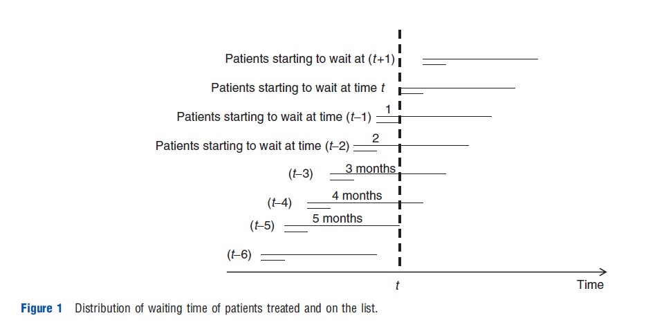
For a given procedure, condition or specialty, two common measures of waiting times can be recorded: (1) the waiting time of the patients on the list at a point in time (or a census date) and (2) the waiting time of patients who have received a treatment (during a predetermined period). The first measure refers to an ‘incomplete’ measure of waiting time as the patient is still on the list (all patients are still waiting): there will be some patients who have just entered the list and some patients who have been on the list for a long time. The second measure refers to the full duration of the waiting-time experience from the time the patient is added to the list to the time the patient is admitted to the hospital for treatment: the measure is computed retrospectively once the wait is terminated.
Figure 1 provides an example which illustrates the difference between the waiting times of the two distributions. In each period two patients enter the waiting list, the first waiting for 1 month and the second waiting for 5 months. In period t only two patients have their wait completed. One has waited for 1 month and one has waited for 5 months. The average wait of patients treated (which is the correct expected wait for the patient) in period t is therefore three periods. At time t there are 6 patients waiting on the list: two patients have waited for one period, one for two periods, one for three periods, one for four periods, and one for five periods. The average wait is therefore 2.7 periods. The key difference between the two distributions is that the distribution of patients on the list tends to ‘‘oversample’’ long-wait patients. Indeed, in the example five out of six are long-wait patients at the time of observation while in fact there is an equal proportion of long and short-wait patients. The reason why in the example the average wait of patients on the list is shorter than the average wait of patients treated is that most of the patients in the list at the time of observation have not completed their wait yet. Hence the data on patients on the list suffers from ‘‘interruption’’ bias. In the present example the interruption bias dominates the long-wait oversampling bias. In Section ‘Waiting Time of Patients on the List Versus Waiting Time of Patients Treated: An Example’ differences between the two distributions are illustrated more formally. An example where the average wait of the patients on the list is higher is also provided.
Waiting Times As A Mechanism To Bring The Healthcare Market To An Equilibrium
A Simple Theoretical Framework
Publicly funded healthcare sectors in many countries are often characterized by zero or little copayments and simultaneously by capacity constraints. If capacity is less than potential demand, this generates an excess demand. If patients in ‘excess’ are added to a waiting list, then patients will have to wait a certain time before receiving treatment.
Economists have argued that waiting times can then be thought of as a price (a non-monetary one), which patients have to pay to access healthcare. In other sectors of the economy, monetary prices bring demand and supply in equilibrium; higher prices reduce demand by discouraging some consumers to buy a certain good and increase supply by encouraging the provider to expand production. Equilibrium prices are determined where the demand curve crosses the supply one. The standard economic demand–supply framework can readily be adapted to the health sector. Like monetary prices are determined such that demand is equal to supply, in the health sector waiting times (the non-monetary price) are determined to bring demand and supply in equilibrium. Note that if demand would systematically be larger than supply, and both demand and supply do not respond to waiting-time variations then the waiting list and the waiting time would keep growing over time.
There are different mechanisms through which waiting times affect the demand for and supply of healthcare (as measured, e.g., by the number of discharged patients). On the demand side, patients may opt for care in the private sector if they are not willing to wait and if they can afford to pay the (monetary) price charged by the private sector. Some patients may also simply give up the (public or private) treatment or opt for a pharmaceutical one. On the supply side, higher waiting times may induce providers to increase activity either because waiting times are used as key performance target (associated with penalties or monitoring) or because providers (doctors) feel bad about patients waiting for a long time.
Perhaps, most importantly when waiting times are higher, policymakers may be willing to allocate more resources to increase the supply of healthcare (although this may also generate perverse incentives if providers artificially inflate the list to attract more resources).
A simple formal model is provided. Define D(w) as the demand for healthcare which depends on the waiting time w. If assumed that higher waiting times reduce demand, then D`(w)<0. Similarly, the supply curve is defined by S(w) with S`(w)>0. In such a market the equilibrium waiting time is determined such that D(w*) = S(w*). The equilibrium waiting time is described in Figure 2 as point A.
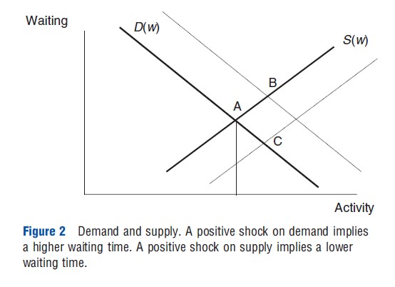
Using this framework, the effect of exogenous shifts on the demand and the supply curve can also be explored. If, for any given waiting time, demand increases (an upward shift in the demand curve) then its equilibrium waiting time and activity will also increase. A higher demand implies that more patients are added to the waiting list, which ultimately leads to an increase in waiting time. Providers will respond to such an increase in waiting time by making more effort to increase activity (point B in Figure 2).
Similarly, if, for any given waiting time, supply increases (a shift to the right of the supply curve) then in equilibrium waiting time will reduce and activity will increase (point C in Figure 2). This shift may be due to an increase in capacity, as measured by an expansion in the number of hospital beds and doctors. A higher supply implies that more patients are taken out from the waiting list, which reduces waiting times; such a reduction is offset to some extent by an increase in demand.
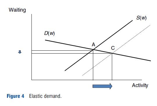
Figure 2 also shows that the responsiveness of demand and supply to waiting times play a crucial role. If demand is very inelastic (nearly vertical, as drawn in Figure 3) an increase in supply will lead to a large reduction in waiting times. In contrast if the demand is elastic (nearly horizontal, as drawn in Figure 4), an increase in supply will lead only to a small reduction in waiting times.
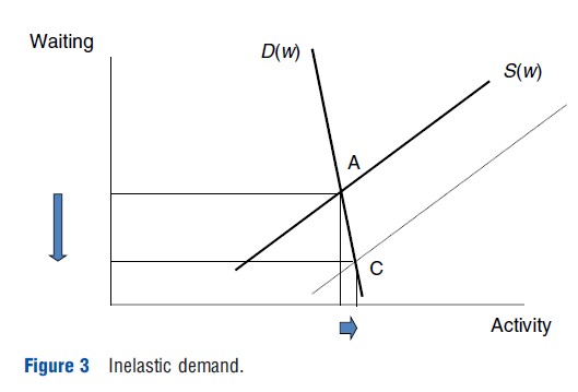
Figures 3 and 4 illustrate a point which is critical in policy discussions on how to reduce waiting times. Some policymakers argue that increasing supply to the health sector will not reduce waiting times because the increase in supply will be offset by an equal increase in demand. As clearly depicted in Figure 4, this type of reasoning implicitly assumes that the demand is elastic. Others argue that a higher supply will bring down waiting times. As depicted in Figure 3, it implies that the demand is inelastic. Empirical estimates of how demand responds to waiting times are therefore paramount to decide whether increasing supply can or not significantly reduce patient waiting times.
Most of the existing empirical estimates of the demand curve from England put the elasticity of demand to waiting time at -0.1 (a 10% increase in waiting times leads to a reduction in demand by 1%). This suggests an inelastic demand curve: higher supply will lead to significant reductions in waiting times (as in Figure 3). It is worth emphasizing however that the existing empirical studies on demand elasticity have been derived mainly for the English healthcare system and should therefore not necessarily be transposed to other countries. One study from Australia, for example, has observed that demand was elastic to waiting times (with elasticity greater than one). Estimates of the supply elasticity even for England vary depending on the study (see discussion below).
Figures 2–4 also show the critical role of demand and supply shifts over time in determining the evolution of waiting times. In the health sector demand tends to increase over time. This is both due to the aging of the population that increases the healthcare needs and also due to technologIcal development, which makes new treatments available (some patients can be treated now who could not be treated in the past). This generates increasing pressures on waiting times. Supply may also increase over time due to the technological advancement that allows treating patients safely with less invasive treatments and a shorter length of stay. Whether waiting times increase or reduce over time depends on the difference between the increase in demand and increase in supply. The gap between demand and supply may also depend on the type of system, with National Health Services being generally associated with tighter capacity constraints, and longer waiting times, than public (or private) insurance systems.
Policymakers have also tools available to influence the demand and supply of healthcare. For example, on the demand side countries with a gatekeeping system (where the patient has to see a family doctor before seeing a specialist) may have lower levels of demand. Moreover, eligibility to public treatment may be made conditional on certain criteria (like severity thresholds, benefits, appropriateness, and cost-effectiveness). More stringent criteria will lead to lower demand. Policymakers may also control the type of technology that is available to hospitals (and e.g. decide not to provide a certain treatment).
On the supply side, policymakers can influence supply by deciding the level of capacity in the public sector (the number of hospitals, doctors, nurses). The payment system for doctors and hospitals will also influence supply with fee-for-service rules and activity-based funding possibly being associated with a higher supply compared with a salary system and fixed budget rules.
Empirical Evidence
Estimates on demand and supply responsiveness to waiting times have been the subject of several empirical studies, mainly with data from England. They have used either a cross-sectional (i.e., a sample of hospitals or small areas at a point in time) or a panel-data (a repeated cross section over time) approach. The cross-sectional approach aims at identifying whether regions with higher waiting times have lower demand, for a given supply, or have higher supply, for a given demand. The analysis can be carried out either at a hospital level (variations across hospitals) or at a small-area level.
One problem with the estimation of demand and supply responsiveness is that separate measurements of demand for healthcare and supply are generally not available. What the researcher can typically observe, say at the hospital level, is different combinations of waiting times and activity levels. The researcher cannot tell whether the different activity levels reflect demand or supply variations.
To disentangle the differential effect of waiting times on the demand and supply of healthcare more sophisticated approaches than Ordinary Least Squares (OLS) need to be implemented. Estimating the responsiveness of the demand function to waiting times by regressing activity on waiting times and demand shifters (e.g., health needs or population) will lead to biased (distorted) results. Similarly, estimating the responsiveness of the supply function regressing activity on waiting times and supply shifters (e.g., the number of doctors and the number of beds) will lead to biased results. The endogeneity of waiting times in determining both demand and supply is typically addressed through the use of one or more ‘instrumental’ variables (a variable that is correlated with waiting times but not the dependent variable). In the demand equation this entails finding a variable that affects waiting times but does not affect the demand: a natural choice is a supply-shifter; for example, more doctors reduce waiting time but have no effect on demand. Similarly, in the supply equation the researcher needs to find a variable that affects waiting times but not the supply. In this case a suitable instrument is one or more demand shifters; for example, a higher proportion of elderly population will be correlated with waiting times but not with the supply.
Using a cross-sectional approach, Martin and Smith (2003) suggest that the elasticity of demand in the English NHS is between 0 and -0.2 depending on the year (-0.2 in year 1991–92, 0 in years 1993–94 and 1996–97, and between – 0.12 and -0.15 in the remaining 4 years). The demand function is therefore inelastic: a 1% increase in waiting time reduces demand by at most 0.2%. In contrast, the supply function is rather elastic: between 2.1 and 5.9 depending of the year considered.
An alternative approach to cross-sectional analysis is the panel-data analysis, which involves data collection on activity and waiting times over several years (say approximately 3–7 years). In this case, the analysis tries to exploit how variations over time for a specific provider affect the demand and supply of healthcare. The results are very much in line with the cross-sectional one with an overall demand elasticity of -0.09 and a supply elasticity of 5.3. The elasticities also vary for different specialties; for example, the demand elasticity is higher (in absolute terms) for general surgery and oral surgery (equal to -0.24 and -0.21, respectively) and smaller for orthopaedics(-0.07).
Waiting Times Versus Waiting List
The above discussion refers mainly to the duration of waiting times and not to the size of the waiting lists. This is for two reasons. First, from the patients’ perspective what matters is how long they wait, and not necessarily how many patients are on the waiting list; if each patient waits for 2 weeks the disutility from waiting is the same regardless of whether there are 100 patients or 1000 patients on the list.
Second, waiting times and waiting lists do not necessarily move in the same direction. To illustrate this point, recall that the number of patients treated in equilibrium is y*=D(w*) = S(w*). Define L as the waiting list. Note that at steady state (when the waiting time and the waiting list do not vary over time), w*=L*/y*. This expression is intuitive; it simply says that the waiting time for a typical patient is equal to the number of periods necessary to treat all the patients on the list. Therefore, if the waiting list has 200 patients and only 10 patients per week are treated, then the waiting time is 20 weeks.
Perhaps less intuitively, the waiting list can be rewritten as the product of activity and waiting time: L*=y*w* . Figure 2 can then again be used to investigate the effect of shocks on the demand and supply side on the waiting list. Figure 2 shows that an exogenous increase in demand increases both equilibrium waiting time and equilibrium activity (compare point A with point B). As the waiting list is the product of the two, then the waiting list will also increase. An exogenous increase in supply instead reduces waiting times and increases activity. The waiting list which in the long run is given by the product of activity and waiting time can then either increase or reduce in response to an exogenous increase in supply (e.g., due to an increase in the number of doctors and beds).
Historically, waiting lists have been initially collected by policymakers as they were more easily available but in recent years a shift in focus on waiting times has been observed.
This section has used a static framework. The Section ‘Waiting Times Dynamics over Long Periods of Time’ expands such framework and allows demand and supply to increase over time driven, for example, by the technological development.
Competition And Choice
Many OECD countries have introduced in the last 20 years hospital payment systems of the Diagnosis Related Groups (DRGs) type where a public insurer (or the government) pays each hospital a tariff for every patient treated with a given diagnosis. This type of system is also known as activity-based financing. Patients typically receive treatment free of charge or are subject to small copayments.
As tariffs are the same across providers (they are regulated), hospitals have to compete on quality and waiting times to attract patients. Policymakers often argue that such competition among hospitals can also be beneficial to reduce waiting times. The intuitive idea is that under a competitive system, the provider will have an incentive to reduce waiting times to attract more patients and ultimately increase hospital revenues.
A prerequisite for implementing such competition policies is patients’ choice; it is only if patients (or family doctors on their behalf) actively compare waiting times and quality across providers that providers will have an incentive to reduce waiting times to attract patients.
The higher the tariff paid to the hospital, the stronger will be the incentive to attract patients. DRG prices are normally based on average-cost rules. However, in some countries, like Norway, the price can be significantly less than the average cost (between 40% and 50%) in which case the incentive is reduced. Moreover, in some cases even countries that make use of DRG pricing have caps on the number of patients treated; the price can be significantly reduced once a certain volume of patients has been reached. In such cases the incentive to compete on waiting times can be significantly reduced.
Whether the hospital has a financial incentive to attract more patients by reducing waiting times depends on the difference between the tariff and the marginal cost. It is only if the profit margin is positive that the financial incentive is present. However, even if the profit margin is positive the provider may still lack the incentive to compete on waiting times. If the number of doctors is fixed and if the demand for treatment is high and there are strict targets on waiting times, doctors may be working at a point where the marginal utility from treating an extra patient is negative. In such cases, the introduction of competition may have an adverse effect on waiting times; intuitively by increasing waiting times, the provider can shift the cost of an unprofitable patient to another provider, which may generate a spiral towards high waiting times. Such results can be derived more formally through the stylized model provided in the Section ‘A stylized Model of Hospital Competition’.
Empirical Evidence
There are two main empirical approaches to test the model outlined above. First, one prerequisite for competition to ‘work’ is that patients are willing to move when waiting times are higher. Empirical studies that model patients’ choice suggest that at least in two countries (England and Norway) patients do react to variations in waiting time but the elasticity with respect to waiting time is low. The results are derived by regressing the hospital’s choice of the patient (measured through a dummy variable equal to one for choosing a given hospital) as a function of waiting times in all hospitals in the catchment area of the patient (e.g., where the patient resides).
A second approach is to focus directly on the relationship between waiting time and competition, regressing waiting time of a given hospital on the number of hospital within the catchment area of the hospital. Using a cross-sectional framework one empirical study finds that in England an increase in competition by one hospital (from five to six hospitals) has a modest effect on waiting times reducing them by half week, from 17 to 16.5 weeks. A different study also tested the effect of competition on waiting times using a natural experiment framework in England: the control group includes providers who are ‘local monopolists’ and have no potential competitors within their catchment area. During 1997–99 competition (the policy of interest) was highly encouraged whereas during 1992–96 market boundaries were assigned geographically. The study shows that the introduction of competition leads to a reduction in waiting times by 0.8 months (see final section for detailed References:).
Waiting Times And The Private Sector
Waiting times play a key role in the interaction between the public and the private sectors. Patients who are not willing to wait for a free public treatment may opt for the private sector paying a fee. Higher waiting times will lead to more patients being treated in the private sector. Anticipating that they will want care in the private sector, higher waiting times may also induce more individuals to buy private health insurance to cover the price charged by the private sector.
The incentive to set waiting times in the public sector may differ when a private sector is present or banned. Without a private sector, a public sector incentive to increase waiting times is such that the probability of idle capacity is optimally minimized. With a private sector a marginal increase in waiting times has the additional benefit (from the public provider perspective) of shifting patients to the private sector, which reduces costs in the public sector. Waiting times may therefore be higher in the presence of a private sector.
The incentive of the public sector to increase waiting times may be reinforced in the presence of ‘dual practice’, that is, when doctors are allowed to work in both the public and the private sectors. An increase in waiting times increases revenues in the private sector and generates a conflict of interest for doctors working in the public sector.
When the public and the private sectors interact, and patients differ in their severity, doctors may have an incentive to cream-skim the patients in the private sector to gain higher profits. Which patients are cream-skimmed depends on the rationing rule used by the public provider and the threshold severity level over which patients are entitled to public treatment. Intuitively, it would be expected that patients with the lowest severity to be cream-skimmed in the private sector. This may not always be the case. Patients with lower severity may not be willing to pay the price charged by the private sector and may also not be eligible for public treatment. Incentives to cream-skim will be highest for patients with middle severity when the severity threshold required for public treatment is high; for those patients severity is high enough to be willing to pay the price in the private sector but not high enough to be eligible for public treatment.
Maximum Waiting-Time Guarantees
In a number of countries, in response to rising waiting times, policymakers have introduced maximum waiting-time guarantees. In its simplest form, a maximum waiting time guarantee says that no patient should wait for more than a predetermined number of months or weeks. This has been the case, for example, in England. Such guarantees are ‘unconditional;’ they hold for every patient regardless of the treatment.
One problem with such unconditional guarantees is that they may conflict with clinical prioritization. As they refer to a maximum, the patients who benefit from this guarantee are likely to be those with a lower priority, who indeed wait the longest. There is therefore a risk that patients with lower severity may be given priority over patients with higher severity, who tend to wait less. Empirical evidence from England suggests that this is indeed the case; the probability of being admitted for treatment increases as it approaches the target but it decreases after the target.
To address this issue, unconditional guarantees have been replaced in some countries (like Sweden in the 1990s) with ‘conditional’ ones where the guarantee is given only conditional on having a certain severity. The maximum waiting time can differ between different severity groups (normally three or four). The most sophisticated form of conditional guarantee is one that specifies a ‘personalized’ waiting time (like in Norway), which depends on several criteria including urgency, benefit and cost-effectiveness from treatment. In contrast to unconditional ones, conditional guarantees conflict less with prioritization (and can actually be seen themselves as prioritization rules). They however suffer from their own limitations: as the provider has discretion over assigning a guarantee to a certain group and a provider can use such discretion to make sure it complies with the guarantee. One possibility to reduce the scope of such discretion is to develop explicit guidelines (though developing a guideline is quite a costly procedure as it involves extensive consultations).
One common problem to maximum waiting-time guarantees is how to enforce them. Although it is quite simple to state that no one or a subset of patients should not wait for more than a predetermined amount of time, it is not clear why the provider should have the incentive to respect such guarantees. The empirical evidence suggests that maximum waiting times work only when they are in the form of targets and clear penalties are attached to them. In England, one study made use of a ‘natural experiment’ to test whether or not a waiting-time target policy combined with sanctions for hospital managers resulted in a reduction of hospital waiting times. Scotland was used as the control group. The study finds that ‘targets and terror’ policy significantly reduced the number of patients waiting more than 6 and 12 months by 20% and 60%, respectively.
Equity Issues
This article has argued in the Section ’Waiting Times as a Mechanism to Bring the Healthcare Market to an Equilibrium’ that waiting times act as a rationing device that brings about an equilibrium to demand and supply. It can also be argued that, despite waiting times generating disutility to patients, one advantage of rationing by waiting is that such form of rationing is equitable because the ability of affording such nonmonetary price does not depend on the ability to pay. This is in contrast to price rationing, for example, in the form of a copayment, which can be more easily afforded by richer individuals.
A recent empirical literature suggests, however, that waiting times may not be as equitable as they appear because individuals with higher socioeconomic status (usually measured by income or educational attainment) tend to wait less, and therefore pay a lower nonmonetary price, in publicly funded hospitals, than patients with lower socioeconomic status. Such gradient is found in separate studies in Australia, England, Norway, and Sweden and may be interpreted as evidence of inequity, which favors the rich and more educated patients over poorer and less educated ones.
One advantage of copayments over waiting times to contain demand, as opposed to waiting times, is that the cost to patients generated by long waiting times is not necessarily recovered by anyone else (except from the reduction in idle capacity that are exhausted quite rapidly). In contrast, copayments raise resources for the provider, which can be recovered by the government. Moreover, copayments could be income tested to address equity concerns though there may be administrative costs associated with it.
A final argument in favor of waiting times is in terms of redistribution. Waiting times induce some better-off patients to opt for the private sector. Patients who opt for the private sector pay twice; they pay the price to receive the treatment in the private sector and also pay taxes, which contribute to the funding of public health systems. If governments have limitations to the extent to which they can redistribute between different income groups, the presence of waiting times may then help to redistribute resources form the rich to the poor (although indirectly).
Conclusions
Waiting times are a pervasive feature of many public-funded healthcare systems and increase with the gap between demand and supply. In future, demand is likely to grow driven by the aging population and by the technological advancements. In contrast, given the current economic climate, there are limits to the extent to which governments can allocate additional resources to increase supply or identify significant efficiency gains. Waiting times may therefore be on the rise. As waiting times generate a significant dissatisfaction among patients and the general public, optimal demand management and patients’ prioritization will play a key role in future policy developments.
Technical Appendix
Waiting Time Of Patients On The List Versus Waiting Time Of Patients Treated: An Example
To illustrate the difference in the distribution of waiting times for the patients on the list versus the distribution in waiting times of patients treated, a simple illustrative example (based on Dixon and Siciliani, 2009) is provided. For expositional clarity, one period is referred to as 1 ‘month.’
Suppose that in each period there is a fixed number of patients who enter the waiting list, which is normalized to one, and an equal number who are treated (therefore a steady state is assumed). Suppose also that the proportion of patients entering the waiting list at any point in time and waiting more than 1 month is p1, so that (1-p1) get treated in the first month. In the second month, conditional of having waited for 1 month, a proportion equal to (1-p2) get treated and p2 keep waiting. By the third month, everyone is treated so that p3=0 or (1-p3) = 1: no patient waits for more than three periods.
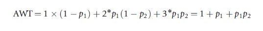
The distribution of the patients treated at any point in time (say in any given month) is the following. There are (1-p1) patients waiting for 1 month, p1(1-p2) waiting for 2 months, and the remaining (p1p2) patients waiting for 3 months. The average waiting time of the patients treated (AWT), measured in months, is therefore
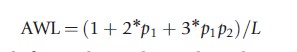
The length of the waiting list at any point in time, denoted by L, is equal to L=1+p1 +p1p2. At any point in time there is a whole cohort of patients (equal to one) who waits for 1 month (i.e. the minimum wait), plus those who started to wait the previous period (equal to p1 as 1-p1 were treated in the previous period) and those who started to wait 2 months before (equal to p1p2). The average waiting time of the patients on the list (AWL) is therefore equal to
It is straightforward to show that the AWT>AWL if (p1(1+p2)2 -p2)p1>0. The comparison is, in general, indeterminate and depends on p1 and p2.
As a numerical example suppose that p1=0.2 and p2= 0.8, which implies that only 20% of the patients keep waiting to the second month, and conditional on having waiting for 1 month, 80% keep waiting for 3 months. Then, AWT=1.32 months and AWL =1.38 months, and the average waiting time of the patients on the list is higher than that of patients treated. The opposite holds if p1=0.4 and p2=0.8.
As the first measure refers to an ‘incomplete’ measure it would intuitively be expected to be shorter than the second measure. This is however not necessarily the case. When looking empirically at the distribution of waiting time it may well be the case that the proportion of patients waiting more than 6 months or the average waiting time for the patients ‘on the list’ is actually larger than those treated. This arises because ‘long waiters’ are overrepresented (or oversampled) under the first measure, which causes the waiting time to go up.
Waiting Times Dynamics Over Long Periods Of Time
This section provides a simple stylized model of waiting-time dynamics, which illustrates the long-run determinants of waiting times. The analysis provided above (and in Figures 2–4) is static as demand and supply depend on waiting times and not directly on time. Changes over time have been analyzed only through exogenous shocks on demand and supply. As argued above, both demand and supply can vary over time possibly at different rates due to the technological development and a range of other factors. A simple way to model time-varying demand and supply function is to assume that they are linear and, respectively, equal to D(w,t)=a+bt -cw and S(w,t)=d+et+fw, where t is the time and a, b, c, d, e, and f are positive parameters. Other parameters a and d can be interpreted, respectively, as demand and supply at time zero when the waiting times are zero; c and f as the responsiveness of demand and supply to waiting times; b and e as the degree at which demand and supply increase over time due, for example, to technology developments. The waiting time dynamics can be formally represented by the following differential equation:
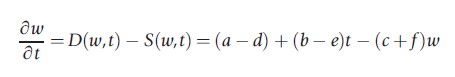
which suggests that waiting times increase over time when demand is higher than the supply and reduce when waiting times are lower than supply. The closed-form solution of the above equation (assuming a = d to keep the exposition simple) is as follows:
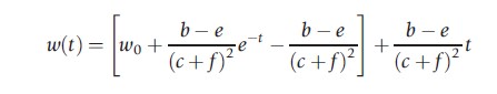
The first term in the square bracket goes to zero as time passes. The long-run dynamics of waiting times is then driven by the difference between b and e, that is, the difference in the speed at which demand and supply grow over time. Intuitively, if demand grows faster than the supply, then waiting times will increase over time. Vice versa, if supply grows faster than the demand, then waiting times will reduce and eventually disappear. The smaller the growth in waiting times, the higher is the response of demand and supply to waiting times.
Given the current economic climate, public budgets allocated to healthcare may reduce or stagnate, and therefore slow down the growth in the supply of healthcare. As a result, waiting times may be on the rise. Policymakers will have to either seek efficiency gains on the supply side or intervene on the demand side to prevent rapid growth of waiting times.
A Stylized Model Of Hospital Competition
Some of the arguments provided in Section ‘Competition and Choice’ can be illustrated through a simple stylized model (adapted from Brekke et al., 2008). Suppose that there are two hospitals i and j. It is assumed that the total demand is inelastic and equal to 1 (which can be thought of as 100% of the patients being treated) and every patient receives treatment in one of the two hospitals. A Hotelling set up is used, which assumes that the two hospitals are located at the extremes of a unit line is used. The demand function of hospital i is given by Di (wi ,wj)=1/2-(wi -wj)/2t, where wi and wj are, respectively, the waiting times in hospital i and j. If waiting times are identical, then each hospital has half of the market. If waiting times are higher in hospital i, then the demand in hospital i is less than half of the market. The parameter t is a transportation (or other) cost parameter, which can broadly be interpreted as the extent to which patients are willing to switch from one provider to the other. Lower transportation costs imply that patients are more willing to switch from one provider to the other when waiting times are lower. This parameter can be influenced by policymakers: making, for example, waiting-time information easily available to patients is equivalent to a reduction in transportation costs.
Assume that the payoff function of the hospital, defined by U, is given by the difference between revenues and the sum of monetary and non-monetary costs, which is given by the following expression:
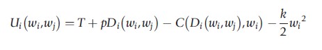
where p is the price for each patient treated, T is a fixed-budget component, C(∙) is the cost function of treating patients (discussed in more detail below), k is a parameter that is proportional to the penalties from having long waiting times (e.g., deviations from waiting-time targets): higher waiting times imply a higher disutility in the form of more monitoring and a higher threat of dismissal for senior managers. To keep the presentation simple assume that the cost function C(∙) is quadratic:
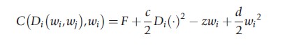
where F is a fixed cost, and c, d, and z are positive parameters. Assume also that a higher activity increases costs at an increasing rate (CDi(∙)=cDi). This cost function captures both monetary and non-monetary costs. As in public hospitals the number of doctors is fixed, it is plausible that the marginal disutility (i.e. the nonmonetary marginal cost) from treating an extra patient is increasing. This specification also allows for the possibility that higher waiting times reduce costs by lowering the probability of idle capacity (Cwi(∙)=-z+dwi ). When waiting times are zero, a marginal increase in waiting reduces costs. However, this happens at a decreasing rate and there may be a point where higher waiting times increases costs due to the higher costs of managing the waiting list.
Differentiating the utility function, the following condition for optimal waiting times is obtained:
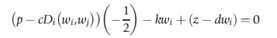
A marginal reduction in waiting times generates benefits and costs. On one hand, it increases activity which generates higher revenues and also makes waiting-times target figures look better. On the other hand, it increases monetary and nonmonetary costs either directly through higher activity or indirectly through higher idle capacity. In the symmetric equilibrium,
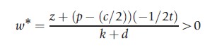
which is always positive whenever the price p is not too high (or the cost c not too low). As expected, stricter targets (higher k) or higher prices p reduce waiting times, and higher costs (c) increase waiting times.
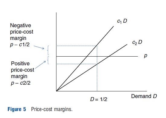
Critically, in equilibrium the price-cost margin (p-(c/2)) can be positive or negative. This depends on the price and the steepness of the marginal cost. Figure 5 illustrates the two possible cases with one price p and two marginal cost curves being characterized by c1>c2 . When the marginal cost is higher (lower), the profit margin is negative (positive).
How does more competition affect waiting times? Policies that encourage competition can be thought of as policies which reduce the transportation costs or the cost of switching between providers. Differentiating the equilibrium waiting time with respect to transportation cost parameter yields the following:
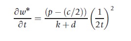
Whether more competition increases or reduces waiting times depends on the price-cost margin (p-(c/2)). More competition (lower transportation costs) reduces waiting times only if the margin is positive (i.e., the price is sufficiently high). In contrast, more competition increases waiting time if the margin is negative (i.e., the price is sufficiently low). The intuition for the latter result is that if providers are working at a negative margin, then under more competition a marginal increase in waiting times becomes more effective in shifting unprofitable patients to the other provider. In contrast, if it is positive a reduction in waiting times attracts profitable patients.
The above analysis assumes that providers are altruistic, which is a realistic and plausible assumption for healthcare providers. Introducing altruism generates two additional effects. On one hand, altruism makes the providers even more willing to work at a negative profit margin, which in turn tends to reinforce the result that competition increases waiting times. On the other hand, altruism induces providers to compete for patients because they can do more ‘good.’ This effect goes in the opposite direction.
References:
- Brekke, K., Siciliani, L. and Straume, O. R. (2008). Competition and waiting times in hospital markets. Journal of Public Economics 92, 1607–1628.
- Dixon, H. and Siciliani, L. (2009). Waiting-time targets in the healthcare sector. How long are we waiting? Journal of Health Economics 28, 1081–1098.
- Martin, S. and Smith, P. C. (2003). Using panel methods to model waiting times for National Health Service surgery. Journal of the Royal Statistical Society 166, 1–19.
- Barros, P. P. and Olivella, P. (2005). Waiting lists and patient selection. Journal of Economics and Management Strategy 14, 623–646.
- Dimakou, S., Parkin, D., Devlin, N. and Appleby, J. (2009). Identifying the impact of government targets on waiting times in the NHS. Health Care Management Science 12, 1–10.
- Gravelle, H., Smith, P. C. and Xavier, A. (2003). Performance signals in the public sector: the case of health care. Oxford Economic Papers 55, 81–103.
- Iversen, T. (1997). The effect of private sector on the waiting time in a National Health Service. Journal of Health Economics 16, 381–396.
- Marchand, M. and Schroyen, F. (2005). Can a mixed health care system be desirable on equity grounds? Scandinavian Journal of Economics 107, 1–23.
- Martin, S. and Smith, P. C. (1999). Rationing by waiting lists: An empirical investigation. Journal of Public Economics 71, 141–164.
- Propper, C., Burgess, S. and Gossage, D. (2008). Competition and quality: Evidence from the NHS internal market 1991–9. The Economic Journal 118, 138–170.
- Propper, C., Sutton, M., Whitnall, C. and Windmeijer, F. (2008). Did targets and terror reduce waiting times in England for hospital care? The B.E. Journal of Economic Analysis & Policy 8(2), (Contribution, Article 5).
- Sharma, A., Siciliani, L. and Harris, A. (2011). Waiting times and socioeconomic status: Does sample selection matter? HEDG Working paper.
- Siciliani, L. and Martin, S. (2007). An empirical analysis of the impact of choice on waiting times. Health Economics 16, 763–779.