Latent Factor and Latent Class Models to Accommodate Heterogeneity

In statistics and econometrics, heterogeneity typically refers to a random variable, parameter, or distribution that varies across a population of interest. It can involve the mean, variance, or other features of a distribution and may arise from observed and unobserved causes.

Observed heterogeneity is variability in an outcome (or dependent variable) attributable to observed predictors (Skrondal and Rabe-Hesketh, 2004). In the simple linear regression model,

heterogeneity in the expected value of the outcome y_i, denoted E[y_i|x_i], is accounted for by the predictor x_i across subjects i=1,y,n. The parameter β₁ quantifies the magnitude of heterogeneity. Random variability in y_i that cannot be explained by xi is denoted by ε_i, the error term, which is assumed to have mean zero and a constant (or homogeneous) variance var(y_i|x_i) = s2. In parametric modeling, the most common distribution assumed for ε_i is a normal or Gaussian distribution, which has many appealing features including characterizing the ordinary least squares (OLS) estimation method.

Now consider a model with two predictors and an interaction effect,

In eqn [2], the effect of a one-unit change in x_1i on E[y_i|x_i] is β₁+β₃x_2i, illustrating that the effect of x­depends on x­. A consequence of effect heterogeneity is that any statement of the effect of x_1i must be accompanied by the value(s) of x_2i at which it is computed and vice-versa. If x_2i is not observed and the model in eqn [1] is estimated, the OLS estimate of β₁ is a weighted average of the true heterogeneous effects of x_1i with respect to the likelihood of each value of x_2i (Angrist, 1998). When x_1i and x_2i are uncorrelated by design (e.g., x_1i is assigned at random in a randomized trial), the OLS estimate under eqn [1] corresponds to the average effect of x_1i over the individuals in the sample, otherwise being more difficult to interpret.

Other forms of heterogeneity are accommodated by relaxing the assumptions of the linear regression model, yielding a wider array of models and possibly requiring specialized estimation methods. For example, if var(y_i|x_i) depends on x_i (directly or via E[y_i|x_i), the assumption of equal variance at all values of the predictors required by OLS is violated. This phenomenon, referred to as heteroscedasticity, may be accommodated in the context of OLS by dividing y_i and x_i by the standard deviation of the residuals, var(y_i|x_i), and then applying OLS (weighted least squares). If var(y_i|x_i) is known, the process is straightforward, otherwise var(y_i|x_i) must be estimated. Point estimates of β that do not account for heteroscedasticity are estimated imprecisely whereas confidence intervals (frequentist inference) and credible intervals (Bayesian inference) are likely to be incorrectly calibrated. When the objective is to estimate a tail probability or quantile (e.g., in immunoassays seeking to determine whether the concentration of a substance in blood serum exceeds a critical threshold), estimation of the variance function is key. Substantial progress on variance function estimation methods has been made in the context of analyzing assays (Davidian et al., 1988; O’Malley et al., 2008).

Unobserved Heterogeneity And Measurement Error

Unobserved heterogeneity, the variability in y_i arising from unobserved sources, cannot be accommodated without much difficulty as direct adjustment for the cause of the heterogeneity is not possible. To illustrate the difficulties that may arise from unobserved heterogeneity, suppose that to relate an individual’s health, y_i, to his/her intelligence quotient (IQ), u_i, but in lieu of u_i, the educational attainment, x_i, is observed. Because u_i is unobserved directly but essential to the model, it is referred to as a latent variable. The situation is represented by the following equations:

where, by assumption u_i is unrelated to(ε_i ,δi)^T , and δ_i is unrelated to ε_i. Equation [3] is a classical measurement error model (Carroll et al., 1995). The observed data regression,

is problematic because x_i is correlated with the error, ε_i=ε_i-β_iδ_i, in violation of the OLS assumption that the predictors are unrelated to the errors. Here x_i is said to be endogeneous. It can be shown that the quantity being estimated by applying OLS to eqn [4] is pβ₁, where p=var(u_i)/(var(u_i)+var(δ_i))<1 is the attenuation factor (Bedeian et al., 1997). Thus, if the heterogeneity in x_i, arising from δ_i is ignored, the estimated coefficient of x_i will be an inconsistent estimator of β₁.

An alternative model arises when u_i varies according to x_i; i.e., u_i = x_i+δ_i , where x_i is independent of δ_i. For example, x_i is the setting of a machine, the control variable, and u_i is the actual level at which the machine operates. This situation, known as Berkson measurement error (Berkson, 1950) is less problematic, at least in linear models, because the OLS estimate of β₁ under eqn [4] is unbiased, and so the only consequence of this form of measurement error is that var(ε_i)≥var(ε_i), which leads to a reduction in statistical power.

Returning to the classical measurement error model, the availability of replicate observations on x_i allows u_i and hence var(δ_i) to be identified, thus enabling an estimate of pβ₁ to be decomposed into estimates of p and β₁. If replicate observations are not feasible or available, an instrumental variable (IV) – a variable z_i that is related to u_i conditional on u_i being unrelated to y_i – facilitates estimation. In the case of linear relationships, the first condition for z_i to be an IV implies u_i=θ₀+θ₁z_i+y_i with θ₁≠0 and u_i being uncorrelated with the random error y_i. Substituting for u_i in eqn [3] yields:

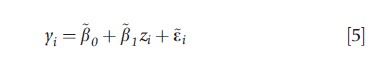
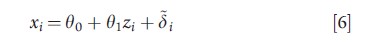
Where β₀=β₀+β₁θ₀, β₁=β₁θ₁, ε_i=β_iy_i+ε_i and δ_i=θ₁y_i+δ_i. Under the second IV condition, z_i is uncorrelated with the errors (ε_i,δ_i)^T, ensuring that OLS yields unbiased estimates of the parameters in eqns [5] and [6]. Hence, consistent estimates of β₀ and β₁ can be deduced from the relations β₀=β₀-(β₁/θ₁)θ₀ and β₁=β₁/θ_1.. Alternatively, one may use two-stage least squares (2SLS): apply OLS to eqn [6] and compute predicted values of x_i, denoted x_i , then apply OLS to eqn [4] but with xi replaced by x_i. The impact of measurement error is a decreasing function of the fraction of variation in xi is explained by z_i. The readers are referred to the article on instrumental variables and to the econometric text by Wooldridge (2002) and that by Angrist and Pischke (2009) for further discussion of IVs, 2SLS, and related methods.

Classic Structural Equation Models

Broadly speaking, a structural equation model (SEM) is a model involving relationships between latent variables. Latent variables generally represent true values of a variable and so relationships between them are often considered to be truisms or causal (Lee, 2007). The use of SEMs to estimate causal relationships has a long history (Pearl, 2000). Latent variables must have associated observed (or manifest) variables in order to identify the model. Traditionally, an SEM is characterized by continuous-valued observed (or manifest) variables, continuous-valued latent (or unobserved) variables, and linear relationships among the latent variables. The linear SEM has the form

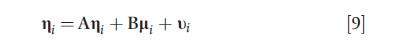
where e_i, δ_i, and u_i are mutually independent error terms with zero means and constant covariance matrices (Joreskog, 1973). Equations [7] and [8] are measurement models relating the observed variables, y_i and x_i, to their latent counterparts, η_i and μ_i, whereas eqn [9] contains the structural model relating the latent construct li to the latent construct η_i. Here Ʌ_y, Ʌ_x and B are matrices of regression coefficients whereas A is a matrix of parameters that affects both the mean and covariance of η_i. The involvement of η_i on both sides of eqn [9] allows for direct relationships between its elements, inducing correlations between them and imposing correlation structure on η_i and thus y_i.

The measurement error model in eqn [3] is a special case of an SEM in which the effect variable is y_i (as observed). Therefore, with replicated measurements, the classic measurement error model in eqn [3] corresponds to y_i=η_i, A=0, B=β₁, and μ₌1u_i, i.e., eqns [8] and [9] reduce to x_i=1u_i + δ_i and y_i=β₁1u_i+ε_I, respectively, where 1 denotes a vector of 1’s. For model identifiability, the dimensions of yi and xi must exceed those of y_i and x_i respectively; the larger the differences, the better. The regression models in eqns [1] and [2] are simple cases of SEMs.

SEMs have been used extensively in the social (e.g., economics, sociology) and behavioral (e.g., psychiatry, psychology) fields. For example, in an analysis of the relationship between job satisfaction and organization commitment to job turnover, Williams and Hazer (1986) use a SEM having the exact forms of eqns [7]–[9]. The measurement models relate observed values of the final outcome (job turnover), intermediate outcomes (intention-to-quit, job satisfaction, organizational commitment), and four exogeneous measures of work environment to their true values. The structural model relates the true values of the outcomes (the endogeneous variables) both to outcomes themselves and to the true values of the work environment variables in order to test hypothesized causal models as depicted by a flow diagram. For a thorough description of the traditional SEM, readers are referred to the classic text by Bollen (1989), the manual of the Linear Structural Relationships (LISREL) software package (Joreskog and Sorbom, 1996), and the recent text by Lee (2007). Modern SEMs extend well beyond linear models, including a wide-range of generalizations of SEMs to outcomes that are not normal (e.g., binary, ordinal, categorical outcomes) (Rabe-Hesketh et al., 2004). Next, models with continuous-latent variables in linear and nonlinear contexts are discussed (see Section ‘Latent Factor Models’), following the same trend for discrete-latent variables (see Section Latent Class and Finite Mixture Models’).

Latent Factor Models

Exploratory factor analysis (EFA) decomposes the covariance or correlation matrix of the centered values (residuals if the model includes covariates) of a sample of multivariate observations by relating these values to a smaller number of latent variables (‘factors’) that are interpreted on the basis of their relationships (‘loadings’) with the observed variables. Among various applications, EFA is used to generate hypotheses with regard to the dimensions underlying the data, to construct summary scales for reporting information, and to eliminate redundant items from questionnaires or survey instruments. The EFA model has the form

where η_iN(0,1), ε_i~N(0,Ψ), 0 is a vector of m zeros, I is an m×m identity matrix, Ψ is a diagonal matrix, and η_i and ε_i are independent vectors of m<r and r random variables, respectively (Johnson and Wichern, 1998). Therefore, cov(y_i,η_i)=Ʌ and var(y_i)=ɅɅ^T+Ψ.

Ambiguity arises with factor decompositions when m>1 as the model is not identified by the data. To illustrate, let T be an m×m orthonormal matrix; i.e., TT^T=I. Then Ʌη_i=ɅTT^Tη_i=Ʌ*η_i*, where Ʌ*=ɅT and η*=T^Tη_i, illustrating that the factor loadings can be ‘rotated’ using an orthonormal basis without changing the fitted values of y_i in eqn [10]. In practice, factor rotation is useful as it provides a means to obtain more interpretable factor loadings. For example, the commonly used factor rotation procedure Varimax seeks to split the factor loadings into two groups, the elements of the one tending toward zero, and the elements of the other toward unity, thereby making it easier to align variables with factors. In an analysis of Joint Committee data on the Accreditation of Health Care Organizations in the US, a hospital level EFA with factor rotation was integral to developing two optimal scales (treatment and diagnosis, counseling and prevention) for the quality of hospitals’ treatment and care delivered to patients with acute myocardial infarction, congestive heart failure, and pneumonia (Landon et al., 2006).

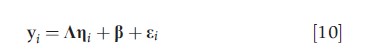
Latent factor models generalize eqn [10] by allowing the expected value of y_i to depend on a matrix of covariates X_i for subject i; i.e.,

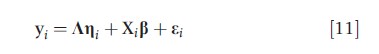
The latent variables η_i are known as latent factors due to the joint dependence of the multiple elements of y_i on the elements of η_i. To identify the model, the variances of the latent variables may be set to 1 (typical in EFA), or an element of each row of K may be set to 1 (typical in latent factor models). The latter anchors the model and makes the variance parameters representative of the strength of the correlation between the outcomes (Skrondal and Rabe-Hesketh, 2004). One of the appealing features of eqn [11] is that model estimation is simplified because the independent assumptions on η_i and ε_i imply that the elements of y_i are conditionally independent given ε_i. Therefore, the distribution of y_i conditional on η_i has the convenient form

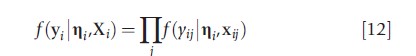
where f(y_ij|η_i,x_ij) is the probability distribution of y_i given η_i. In SEM terminology, latent factor models are measurement models in which the outcomes are directly affected by covariates and jointly dependent on shared latent traits. Because η_i is in the model for outcome j (j = 1,…,r), models that factorize like eqn [12] are referred to as shared-parameter models (Vonesh et al., 2006; Reich and Bandyopadhyay, 2010). In practice, there may be little interest in the factor structure, in which case if m>1, the nonuniqueness of the fitted model is a nuisance. A simple uniqueness condition such as Ʌ^TΨ^-1Ʌ=D, where D is a diagonal matrix, may be imposed to identify the model.

Latent factor models are being used increasingly in applications involving complex data and study designs and, therefore, apply to a broader array of settings than EFA. For example, Hogan and Tchernis (2004) used a latent factor to obtain a model-based index of material deprivation at the census tract level in Rhode Island. They supposed that for each area on a map, four manifest variables (standardized to z-scores) are conditionally independent given a one- dimensional latent factor with spatial correlation incorporated through the latent factor. The model was fit using Bayesian methods and the model-based material deprivation index was defined as the posterior expectation of the latent factor given the observed data. A model-based index confers several ad-vantages over ad hoc methods of combining indices into a single score, including optimally weighting the constituent indices and the computation of their inferences.

Hierarchical Models

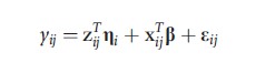
Latent factor models accommodate clustered data and longitudinal data. To illustrate, the authors have presented the latent factor model in terms of individual observations

where j denotes measurement type (ordered the same across subjects), and λ^T_j and x^T_ij are the jth rows of Ʌ and X_i respectively. The random intercept model

where η_i~N(0,τ²) is then seen to be the special case of the latent factor model in which λ_j= 1, a scalar, j = 1,…,m. The importance of the latent factor is quantified by τ²; larger variances are indicative of individuals that differ extensively in unmeasured ways (widely varying η_i). The random intercept–random slope model

is a latent factor model with known factor loadings if z_ij = z_j; i.e., the covariates with random coefficients are balanced in that they do not vary across subjects. Balanced covariates for the random effects may arise when each subject is evaluated by the same set of raters (e.g., radiologists evaluating images) or, in a longitudinal setting, when observations are made at regular intervals. Regularly spaced longitudinal data is common. For example, participants in a study are examined weekly; the Federal Reserve sets interest rates quarterly; quarterly financials are released by companies.

In hierarchical models, latent variables can be incorporated at multiple levels to account for correlation within clusters (Raudenbush and Sampson, 1999). For example, in a study of academic achievement, students may be nested within classes and classes are nested within schools. A hierarchical latent factor model contains latent factors at one or more levels of the hierarchical structure.

Multivariate Mixed Outcome Models

A natural extension of the latent factor model is ascribed to situations where the outcome variables have mixed types (Dunson, 2000). Under the decomposition in eqn [12], a generalized linear model is used to model y_ij with the link function

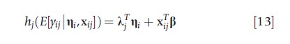
where h_j(·) is a monotone function that maps its argument to an unrestricted random variable. For example, in medical device trials of coronary-artery stents, the key outcomes often include a clinical (binary) and an angiographic (continuous) outcome, leading to one binary and one linear equation (O’Malley et al., 2003). The logit link function was used for the binary component (the probit link would have been an alternative) whereas the linear link (or identity function) was used for the continuous outcome. Other common link functions (associated data types) include the logarithmic link (count data, nonnegative data such as costs or expenditures, time-to-event or survival data) and the log–log link (extreme-event or maximal-outcome data such as in flood prediction).

For discrete-valued (e.g., binary, count) outcomes, additional identifiability constraints are required as the mean and variance are no longer free parameters. However, it is important not to inadvertently restrict the parameter space of the model when imposing identifiability conditions. As a general rule, λ_j should only be constrained if the variance of outcome j is determined by its mean (e.g., as for a binary random variable), in which case setting λ_j=1 is appropriate. But when applied, such an identifying constraint can lead to insolvable identifying conditions (e.g., equations that can only be solved by allowing a variance to be negative).

Joint modeling of multiple outcomes may yield more precise results than separate analyses as information on one outcome can be brought to bear on the analysis of another outcome. However, if the sets of covariates depend on the information by which two outcomes are found to be identical, then point estimates are minimally affected, and unaffected for all outcomes in the case of linear models (Teixeira-Pinto and Normand, 2009).

In a related family of models, the covariates may be modeled through the latent variable (Sammel et al., 1997). Therefore, the coefficients of the covariates are proportional across outcomes and thus represent overall associations with the underlying construct generating the data (O’Malley et al., 2003). Although such proportionality makes it easier to summarize the impact of a covariate, it might be too restrictive in many applications. Furthermore, the regression coefficients affect the marginal variance of the outcomes, because of which estimates are more sensitive to the correlation structure than under eqn [13].

Joint Models Involving Censored Or Missing Data

In longitudinal analyses where outcomes may be censored due to death, the censoring mechanism is nonignorable (i.e., informative) if unobserved factors are correlated with those outcomes that are correlated with survival. One approach for overcoming this problem is to jointly model the outcome and survival time, conditioning on a latent factor to account for unmeasured common causes (Vonesh et al., 2006).

The above approach may be adapted to account for missing values of the outcome (or potentially of covariates) in other contexts. In general, if the number of distinct missing data patterns across the sample is small (e.g., if the outcome is the only variable ever missing, there are only two missingness patterns), missing data can be modeled using a categorical random variable that is the subject of one (set of) equation(s) whereas the outcome is the subject of another equation, both equations depending on observed predictors and a latent factor (Tsonaka et al., 2009). Shared-parameter models provide one of the few methods applicable when the missing data mechanism is not-missing-at-random (Little and Rubin, 2002). For example, in the case when the outcome is the only variable with missing values, a binary regression equation relates d_i= I (y_i =missing) to the observed covariates and a latent variable whereas a second model relates the nonmissing values of y_i to d_i, the observed covariates and the same latent variable.

In observational studies, latent factor models may be used to account for unmeasured confounders affecting the selection of treatment and the outcome. In place of a censoring or missing data indicator, a problematic (i.e., endogeneous) predictor is modeled in conjunction with the outcome. Therefore, models to account for nonignorable treatment selection emulate SEMs by modeling the relationships between latent variables and, like the measurement error model in the Section ‘Unobserved Heterogeneity and Measurement Error’, these models involve simultaneous equations. This scenario is expanded in the Section ‘Bivariate Probit Type Models’.

Categorical Outcome Variables

When the outcomes under the model in eqn [13] have the same form but are binary (or ordinal) as opposed to continuous, the model reduces to an item response theory (IRT) model. The most common IRT model assumes a single latent factor with r categories, x_ij= (I(j=1),..,I(j=r))^T , and a logit link:

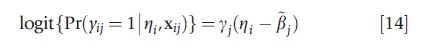
where β_j=β_j/y_j. Thus, the model includes an intercept and slope parameter for every measurement type (e.g., a type of test) along with a single underlying latent variable for each subject (e.g., true level of ability). The specification of the model in eqn [14] is completed by assuming η_i is normally distributed. The same form of model is commonly used to model ordinal responses (see article on models for ordered data).

Although eqn [14] generalizes to allow an m-dimensional latent factor, it is rare to have more than two dimensions. If η_i is treated as a fixed effect parameter, then eqn [14] is the wellknown Rasch model (Rasch, 1960), often used in education or other situations where multiple informants provide ratings of an individual (Horton et al., 2008).

Bivariate Probit Type Models

An alternative to the method in Section ‘Categorical Outcome Variables’ for modeling when outcomes are not normal is to define latent continuous variables y*_ij that underlie a discrete-valued y*_ij. The multivariate normal latent factor model is assumed for y . The bivariate probit is an example of this type of model. Let y_i1 and y_i2 denote binary realizations of underlying normally distributed random variables y*_i1 and y*_i2 respectively. The bivariate probit model can then be defined as

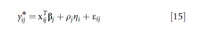
where y_ij=I(y*_ij>0) for j=1,2 and p­=1 for identifiability. The latent factor η_i denotes an unmeasured confounding variable and p*=p₂/(1-p₂²)^0.5 is a measure of the extent of confounding (the selection effect) standardized to [–1,1]. In the absence of covariates, p* is the correlation between two continuous random variables that are estimated from observing two binary realizations, commonly referred to as a tetrachoric correlation (Bonett and Price, 2005). A p*>0 indicates that unobserved factors are such that larger values of y*_i2 are associated with larger values of y*_i1. Bivariate probit models are often used when observations of a binary outcome are available only for a subset of individuals in a study. For example, in a study of the impact of financial incentives on quality of care delivery by physicians, a quality indicator may be available only for individuals with certain health experiences. Whenever a quality measure for an individual depends on unmeasured factors possibly relating to quality of care, then a bivariate model can be fit to account for nonrandom selection into the sample. The outcome equation is augmented with a latent variable that being also a predictor in an equation, describes the likelihood that individual with certain characteristics is sampled. If the regression equations and the probability distribution of the observations are correct, unbiased estimates of the effects of interest (in this case, physician financial incentives) are obtained.

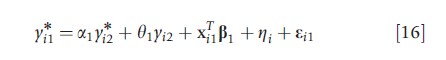
A generalization of the bivariate probit in eqn [15] yields the family of models developed in Heckman (1978), in which one or both of y*_i1 and y*_i2 may be observed, y*_i2 may be a predictor of y*_i1 and vice-versa, and _yi2 may be a predictor of y*_i1 and y*_i2:

The model in eqn [16] accommodates both continuously valued and discrete-valued endogeneous variables, the latter being referred to as a structural-shift. In general, for the model to be identifiable, restrictions on the parameters are needed. The special case of a₁=a₂₌θ₂=0 (all predictors observed) is a parametric alternative to nonparametric IV methods when the endogeneous predictor is binary. In addition, if y is observed but y is not observed, the Heckit model (Arendt and Holm, 2006) arises. If θ₁= θ₂=0 and y*_i1 and y*_i2 are observed, a linear simultaneous equations model is obtained. The article on discrete outcomes includes a detailed review of discrete outcome models with endogeneous predictors.

Latent Class And Finite Mixture Models

In many applications, the study population can be decomposed into a finite number of distinct groups with respect to a variable, y_i. If the variability in the data arises primarily from differences between groups rather than those within groups, the marginal distribution of y_i can be represented by a mixture of distributions of the same parametric form but with unique parameters, {θ_k}_1:K:

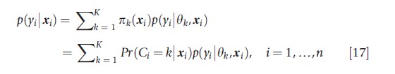
where π_k(x_i)=Pr(C_i=k|x_i) is a latent class probability or mixing weight associated with latent class k, and C_i indicates, conditional on subject i having covariates xi, the subpopulation k (k =1,….,K) to which subject i belongs.

The model in eqn [17] is referred to as a finite mixture model, a latent class model (because it partitions subjects into one of K latent classes), or a discrete-latent variable model (because C_i denotes a latent variable with a finite number of values). When x_1i is observed and x_2i is a discrete-valued unobserved covariate, the interaction effect model in eqn [2] is a latent class model (i.e., the coefficient of x_1i takes on different values across the latent classes that are defined by the unobserved x_2i).

Latent class models are useful when the research goal is to cluster patients into distinct subpopulations, or if one believes that the data-generating process can be modeled by first assuming that subjects fall into one of K latent classes; then, conditional on class-k membership, the outcome y_i is drawn from p(y|θ_k) for subject i. When xi only consists of the scalar 1, eqn [17] assumes that the class-membership probabilities are identical for all n subjects – that is, Pr(C_i=k|x_i) = π_k for all i – and the model reduces to the model-based clustering approach of Fraley and Raftery (2002). In general, however, these probabilities vary as a function of subject-level predictors, x_i. In this case, the class-membership probabilities are typically assumed to follow a multinomial logit or multinomial probit model.

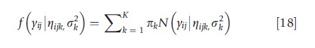
As an illustration, consider a hypothetical study in which y_i denotes the annual medical expenditures for the ith patient. Suppose, further, that the investigators propose to model the data using the following two-component mixture of normal distributions:

where π denotes the probability of class-2 membership and N(μ_k ,σ²_k) denotes a normal distribution with mean μ_k and variance σ²_k(k=1,2). Note that μ₂>μ₁ implies that the mean expenditures for class 2 are higher than those for class 1. Further, σ²₂>σ²₁ implies that class 2 is more dispersed than class 1. Then subjects for whom π>0.50 are more likely to be in a class characterized by high average spending and increased variability relative to class 1. A comprehensive review of latent class models is given in the texts by McLachlan and Peel (2000) and Fruhwirth-Schnatter (2006). In the remaining part of this section, four types of latent class models have been considered.

Latent Growth Models

Latent class models can be applied to longitudinal and clustered data. In the longitudinal setting, the classes are characterized by average trajectories (or ‘growth curves’) over time. Consequently, these models are often referred to as latent growth models (LGMs). For example, a basic linear LGM for a normal outcome variable would take the form:

where η_ijk= β_0k +β+t+and y_ij denotes the response at observation j for individual i; t_ij denotes the time (e.g., from baseline) of the ijth observation; β_0k and β_1k denote the intercept term and the trajectory slope for class k respectively; and σ²_k is the class-k variance of y_ij. Such models presume the existence of an unobserved discrete-valued variable that has both a main effect and an interaction effect with t_ij on the outcome. If the discrete-valued variable is observed, then eqn [18] reduces to a linear regression model with both main effects and time-interaction effects as yielded by the levels of that variable. Therefore, the defining feature of the latent growth model in eqn [18] is that the class to which an individual belongs is a discrete-valued latent variable that is unknown.

Extensions to nonlinear trajectories are straightforward. LGMs are especially popular in developmental psychology, where they have been used to model the progression of physical violence (Nagin and Tremblay, 1999) and criminal behavior (Roeder et al., 1999). They have also been applied to joint longitudinal outcome–survival models (Lin et al., 2002), where latent factor models are an alternative to the shared-parameter model approach to censored or missing data.

Growth Mixture Models

LGMs can be broadened to include subject-specific random effects. Such models are called growth mixture models (Muthe´n et al., 2002) or heterogeneity models (Verbeke and Lesaffre, 1996). Growth mixture models assume that individuals are first placed into one of K latent classes that are defined by a mean trajectory curve (as in LGMs); then, around these mean trajectories, individuals are given their own subject-specific trajectories that are defined by a set of random effects with class-specific variance parameters. As such, growth mixtures can be viewed as finite mixtures of random effect models.

To continue with our previous example, the authors can extend the model in eqn [18] to include subject-specific intercept and slopes:

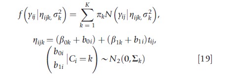
where b_0i and b_1i denote, respectively, a random intercept and random slope for subject i. Conditional on subject i belonging to class k (i.e., C_i =k), the vector (b_0i, b_1i)` is assumed to follow a bivariate normal distribution with mean 0 = (0,0)` and class-specific covariance matrix ∑_k. Growth mixture models have been applied in various contexts, including studies of class-specific prostate specific antigen trajectories (Lin et al., 2000), daily affect (i.e., emotional expression) scores (Elliott et al., 2005), and mental health expenditures (Neelon et al., 2011).

Causal Inference Via Latent Class Models

Latent class models have similarities with the principal stratification approach to causal inference (Frangakis and Rubin, 2002). The connection is illustrated in the context of a randomized controlled trial compromised by noncompliance. A subject’s compliance status is formulated as a categorical variable with four levels on the basis of compliance behavior of the subject under both potential treatment assignments (Frangakis and Rubin, 1999). Under both assignments, compliers take the assigned treatment, always-takers take the experimental treatment, never-takers take the control, and defiers take the opposite treatment to that assigned. For example, in a randomized trial comparing the efficacy of two antipsychotics for refractory schizophrenia, compliers might be defined as individuals who would take the assigned treatment for the entire follow-up period whereas the other three groups characterize those individuals who would switch treatment under one (alwaysand never-takers) or both (defiers) treatment assignments (O’Malley and Normand, 2005). Because compliance status does not depend on the outcome, the same definitions would apply to a health economic outcome such as aggregate mental health cost of treatment. In general, compliance status can be considered as a latent class because it is unobserved (compliance behavior is observed only under the assigned treatment) and the expected outcome from treatment may vary with compliance status (compliers form one principal stratum, never-takers form another stratum, etc.). Thus, a model such as that in eqn [17] could be used. However, in causal inference, the more common approach is to identify the model by imposing structural assumptions as opposed to parametric assumptions, which cannot be completely tested from the data. It is typically assumed that defiers do not exist, an assumption referred to as monotonicity, and that treatment assignment only affects outcomes through the treatment received, the exclusion restriction. Unbiased nonparametric moment-based estimators are then available for the effect of the treatment received on the outcome. In this sense, treatment assignment is an instrumental variable and, under the additional assumption that one individual’s treatment does not affect another’s outcome (the stable unit treatment value assumption), the estimand is a local-average treatment effect (Angrist et al., 1996).

Model Fitting

Two techniques that are especially well-suited to estimation of models with latent variables are the expectation-maximization (EM) algorithm for frequentist inference and Markov-chain Monte Carlo (MCMC) for Bayesian inference. Their suitability arises from the fact that the values of latent variables (continuous-latent factors or categorical latent classes) can be considered as the missing data. Estimation for latent factor and latent class models proceeds by treating the latent variables as missing data and applying either the EM algorithm (Dempster et al., 1977) or, in the Bayesian context, MCMC (Gelfand and Smith, 1990).

EM and MCMC computations can be conceptualized as applying a regular regression (linear or otherwise) on the basis of imputed values of the latent variables (the complete data analysis) and subsequently using all of the information in the data as well as the fitted model to impute the latent variables. In the second step, the EM algorithm yields ‘best’ values of the latent variables by maximizing the complete data likelihood function whereas the MCMC algorithm yields random realizations of the latent variables from the corresponding joint posterior distribution (also referred to as data augmentation) (van Dyk and Meng, 2001).

Prior Distributions For Bayesian Modeling

To fit a Bayesian model, prior distributions need to be specified for the model parameters that have not already been assigned probability distributions (essentially all parameters other than the latent variables). As for the regression coefficients of the observed predictors, the coefficients of the latent factors (the factor loadings) are often assigned normal distributions. When the outcomes y_i or their unobserved continuous counterparts (e.g., in the bivariate probit model) follow a normal distribution, a normal prior yields a normal posterior distribution, which simplifies the MCMC procedure by allowing posterior samples to be drawn directly. However, unless the parameters are restricted to ensure that the model is identifiable, the computational issues discussed in the Section ‘Computational Challenges’ can hinder convergence of model fitting algorithms. An advantage of Bayesian modeling is that prior distributions can often easily accommodate constraints for making the model identifiable by data. For example, in an analysis of monthly international exchange rates, Lopes and West (2004) specify independent normal priors for the factor loadings with two restrictions: the loadings above the diagonal are 0 (thus the factor loading matrix is block lower triangular); and the diagonal elements are nonnegative.

In the latent class model, the class prevalence or mixing probabilities, the pks, are typically assigned a Dirichlet prior, which leads to a convenient closed-form conditional posterior distribution. Covariance matrices are often assigned inverse-Wishart prior distributions or variants thereof, although alternative specifications are becoming more common (O’Malley and Zaslavsky, 2008).

Computational Challenges

Several numerical challenges that arise in fitting SEMs, inclusive of latent factor and latent class models, are due to the fact that the parameterization of latent factor and latent class terms being permuted without affecting the fitted model. This problem is partly resolved in the latent factor case through the use of a uniqueness condition (see Section ‘Latent Factor Models’). However, under MCMC estimation, a related problem called label-switching (Stephens, 2000) arises when the order of the factors varies across the draws from the joint posterior distribution, in which case, posterior summaries resulting from naıve Monte Carlo averages will be nonsensical. To enable inference concerning latent factors, postprocessing is necessary in order to obtain a consistent order of the factors across the posterior draws before computing posterior summaries. Post-processing may also be applied to the draws of the latent class parameters to account for the possibility that ‘Class 1’ in one draw is ‘Class 2’ in another, corresponding to equivalence classes at which the likelihood function has equal maximal values.

Software for implementing latent factor and latent class models includes Mplus, Latent Golds, WinBUGS, and R packages for specific families of models. The SAS procedure Proc Traj fits LGMs for panel data, including whenever observation times are unevenly spaced (Jones and Nagin, 2007).

Model Comparison And Checking

A general way of comparing single-level models (models that do not include random effects or latent variables) is the Akaike Information Criterion (AIC) or the Bayesian Information Criterion (BIC), also known as the Schwarz Criterion. The AIC and BIC balance the level of fit (quantified in terms of the loglikelihood) with model complexity (a penalty for using the sample data to estimate the model parameters). A challenge in applying these methods to SEMs lies in the estimation of latent variables and their effects wherein amounts of information (i.e., degrees-of-freedom) being used are different from those utilized during the estimation of observed predictors and their effects. Therefore, assessing model complexity on the basis of the number of estimated parameters is not appropriate.

In Bayesian analysis, model comparison on the basis of Bayes factors (Kass and Raftery, 1995) is the most principled approach though computational problems may be encountered. Because Bayes factors rely on the marginal likelihood of the data under a presumed model, they only exist if the prior on the model parameters is proper. To allow the use of improper priors, an alternative to Bayes factors, such as the intrinsic Bayes factor (Berger and Pericchi, 1996) has been proposed. The pseudo Bayes factor (Gelfand and Dey, 1994) offers a computationally convenient numerical approximation but has been criticized due to its dependence on the harmonic mean (Neal, 2008). An alternative to Bayes factors is the Deviance Information Criterion (DIC) (Spiegelhalter et al., 2002), which can be regarded as a Bayesian counterpart to the AIC. In response to ambiguity over the appropriate way of accounting for latent variables in finite mixture models, Celeux et al. (2006) have proposed several alternative DIC measures with improved inferential properties. However, discerning and implementing the appropriate measure of DIC is not straightforward in many situations.

Once a model is selected, Bayesian posterior predictive checks can be used to compare the observed data to the one replicated from the posterior predictive distribution under the model (Gelman et al., 1996). If the model fits well, the replicated data would resemble the observed data. To quantify the degree of similarity, the percentile of the predictive distribution corresponding to the observed value of a discrepancy measure that reflects an aspect of model-fit important to the area of study is evaluated. If the percentile, a Bayesian predictive pvalue, is near 0 or 1, the model exhibits lack-of-fit. For more details of Bayesian model specification, model fitting, and model checking, refer to the article on Bayesian analysis.

Limitations Of SEMs

One of the most common criticisms of models involving latent variables is that model identifiability stems from the distribution specified for unobserved variables. Because such assumptions cannot be completely tested by the data, there is a concern that models with latent variables are unscientific. This is of particular concern in models involving structural assumptions such as instrumental variable assumptions. Such concerns have motivated research on nonparametric and semiparametric methods (Lee, 1995), including alternatives to parametric hierarchical (or mixed effect) models (Heagerty and Zeger, 2000).

In studies involving structural assumptions, deciding between nonparametric and parametric SEMs entails a trade-off between assumptions. For example, in IV analyses, the tradeoff is between identifiability of model parameters via the exclusion restriction (typically supported by a theoretical model and, in the case of multiple IVs, partially tested empirically using a test of over-identifying conditions) or via the joint probability distribution of the outcome variable and the endogeneous predictor (O’Malley et al., 2011). In practice, one approach may be a sensitivity analysis for the other.

Summary

The intersection of heterogeneity and SEM encompasses a diverse range of models. Before concluding, several models that are equally important though more loosely connected to the central theme of this article are mentioned. These include two-part models and spatial models. Two-part models account for outcome distributions having multiple parts, distributional heterogeneity. For example, when analyzing medical costs, it is often the case that the outcome distribution is part discrete (zero costs arising when no service is performed) and part continuous (a broad range of nonzero costs associating with different services). Such ‘semi-continuous’ data may be modeled using two-part models with one component of the model being dedicated to the likelihood that the outcome (e.g., cost) is 0 while the other one to the expected outcome of being nonzero (Neelon et al., 2011; Olsen and Schafer, 2001). For more details, refer to the article on modeling expenditure and utilization data.

Analogous models exist for zero-inflated count data. One such model is the Poisson hurdle model, which is a twocomponent mixture consisting of a point mass at zero, followed by a truncated Poisson for nonzero observations (Mullahy, 1986). Other count distributions, such as the negative binomial, can alternatively be used. A related model is the zeroinflated Poisson (ZIP) model, which consists of a degenerate distribution at zero and is mixed with an untruncated Poisson distribution (Lambert, 1992). The ZIP partitions the zeroes into two types: ‘structural’ zeroes (e.g., those that occur because patients are ineligible for health services) and ‘chance’ zeroes (e.g., those that occur by chance among eligible patients) (Neelon et al., 2010). For more details on modeling count data, refer to the article on modeling ordinal outcomes.

In spatial analysis, heterogeneity refers to how a variable yi varies across a region of space. Two common types of spatial data are point-referenced data and areal data. For point-referenced data, yi is measured at a set of geo-referenced locations, s, and the covariance of yi at locations s1 and s2 is assumed to be a function of the distance between s1 and s2. For areal data, the spatial unit is an aggregated region of space, such as a Census block or a county, and yi is typically a count or average response among individuals residing in that region. Popular models for analyzing areal data include the simultaneously autoregressive (SAR) and conditionally autoregressive (CAR) models. Foundational work in the field of spatial modeling has been conducted by Whittle (1954) and Besag (1974). The field of spatial econometrics includes a literature on network autocorrelation as well as other models for the sake of estimating peer effects (Anselin, 1988).

In line with the general emphasis in the statistics and econometric literature, our focus has been on models for the mean (or transformations thereof). One of the few exceptions are mixed effect location-scale models, where the variance as well as the mean of the outcome depends on latent variables (Hedeker et al., 2009). Such models allow shrinkage to an overall variance in addition to shrinkage to an overall mean.

Although it is always possible to specify SEMs by writing out a series of equations or a path diagram, the recent explosion in computing power and development of computer software programs to harness this power have made it possible to fit a wide range of models. This has enabled many extensions to traditional models including accounting for missing data, clustered or hierarchical data, and other heterogeneous features of models to be accommodated. SEMs can yield powerful improvements over traditional approaches to regression, covariance decomposition (or factor) analysis, grouping (or clustering) subjects, and separating cause from association. In the future, the authors predict that the uptake of SEMs will continue to expand into new areas of application.

References:

1. Angrist, J. D. (1998). Estimating the labor market impact on voluntary military service using social security date on military applicants. Econometrica 66, 249–288.
2. Angrist, J. D., Imbens, G. W. and Rubin, D. B. (1996). Identification of causal effects using instrumental variables. Journal of the American Statistical Association 91, 444–455.
3. Angrist, J. D. and Pischke, J.-S. (2009). Mostly harmless econometrics: An empiricist’s companion. Ch. 4. Princeton, NJ: Princeton University Press.
4. Anselin, L. (1988). Spatial econometrics: Methods and models. Dordrecht. The Netherlands: Kluwer Academic Publishers.
5. Arendt, J. N. and Holm, A. (2006) Probit models with dummy endogenous variables. CAM Working Papers. Available at: http://EconPapers.repec.org/ RePEc:kud:kuieca:2006_06 (accessed 17.04.13).
6. Banerjee, S., Carlin, B. and Gelfand, A. (2004). Hierarchical modeling and analysis for spatial data. Chapman and Hall: Boca Raton, FL.
7. Bedeian, A. G., Day, D. V. and Kelloway, E. K. (1997). Correcting for measurement error attenuation in structural equation models: Some important reminders. Educational and Psychological Measurement 57, 785–799.
8. Berger, J. O. and Pericchi, L. R. (1996). The intrinsic Bayes factor for model selection and prediction. Journal of the American Statistical Association 91, 109–122.
9. Berkson, J. (1950). Are there two regressions? Journal of the American Statistical Association 45, 164–180.
10. Besag, J. (1974). Spatial interaction and the statistical analysis of lattice systems (with discussion). Journal of the Royal Statistical Society, Series B: Methodological 36, 192–236.
11. Bollen, K. A. (1989). Structural equations with latent variables. New York: Wiley.
12. Bonett, D. G. and Price, R. M. (2005). Inferential methods for the tetrachoric correlation coefficient. Journal of Educational and Behavioral Statistics 30, 213–225.
13. Carroll, R. J., Ruppert, D. and Stefanski, L. A. (1995). Measurement error in nonlinear models. New York: Chapman and Hall.
14. Celeux, G., Forbes, F., Robert, C. P. and Titterington, D. M. (2006). Deviance information criteria for missing data models. Bayesian Analysis 1, 651–674.
15. Davidian, M., Carroll, R. J. and Smith, W. (1988). Variance functions and the minimum detectable concentration in assays. Biometrika 75, 549–556.
16. Dempster, A. P., Laird, N. M. and Rubin, D. B. (1977). Maximum likelihood from incomplete data via the EM algorithm. Journal of the Royal Statistical Society: Series B 39, 1–38.
17. Dunson, D. B. (2000). Bayesian latent variable models for clustered mixed outcomes. Journal of the Royal Statistical Society: Series B 62, 355–366.
18. van Dyk, D. A. and Meng, X.-L. (2001). The art of data augmentation. Journal of Computational and Graphical Statistics 10, 1–50.
19. Elliott, M. R., Gallo, J. J., Ten Have, T. R., Bogner, H. R. and Katz, I. R. (2005). Using a Bayesian latent growth curve model to identify trajectories of positive affect and negative events following myocardial infarction. Biostatistics 6, 119–143.
20. Fraley, C. and Raftery, A. E. (2002). Model-based clustering, discriminant analysis, and density estimation. Journal of the American Statistical Association 97, 611–631.
21. Frangakis, C. E. and Rubin, D. B. (1999). Addressing complications of intention-to-treat analysis in the combined presence of all-or-none treatment-noncompliance and subsequent missing outcomes. Biometrika 86, 365–379.
22. Frangakis, C. E. and Rubin, D. B. (2002). Principal stratification in causal inference. Biometrics 58, 21–29.
23. Fruhwirth-Schnatter, S. (2006). Finite mixture and Markov switching models. New York: Springer.
24. Gelfand, A. E. and Dey, D. K. (1994). Bayesian model choice: Asymptotics and exact calculations. Journal of the Royal Statistical Society, Series B 56, 501–514.
25. Gelfand, A. E. and Smith, A. F. M. (1990). Sampling based approaches to calculating marginal densities. Journal of the American Statistical Association 85, 398–409.
26. Gelman, A., Meng, X.-L. and Stern, H. (1996). Posterior predictive assessment of model fitness via realized discrepancies. Statistica Sinica 6, 733–760 (Discussion: pp. 760–807).
27. Heagerty, P. and Zeger, S. (2000). Marginalized multilevel models and likelihood inference (with discussion). Statistical Science 15, 1–26.
28. Heckman, J. J. (1978). Dummy endogenous variables in a simultaneous equation system. Econometrica 46, 931–960.
29. Hedeker, D., Demirtas, H. and Mermelstein, R. J. (2009). A mixed ordinal location scale model for analysis of ecological momentary assessment (EMA) data. Statistics and Its Interface 2, 391–401.
30. Hogan, J. W. and Tchernis, R. (2004). Bayesian factor analysis for spatially correlated data, with application to summarizing area-level material deprivation from census data. Journal of the American Statistical Association 99, 314–324.
31. Horton, N. J., Roberts, K., Ryan, L., Suglia, S. F. and Wright, R. J. (2008). A maximum likelihood latent variable regression model for multiple informants. Statistics in Medicine 27, 4992–5004.
32. Johnson, R. A. and Wichern, D. W. (1998). Applied multivariate analysis. Ch. 9. Upper Saddle River, NJ: Prentice-Hall.
33. Jones, B. L. and Nagin, D. S. (2007). Advances in group-based trajectory modeling and an SAS procedure for estimating them. Sociological Methods and Research 35, 542–571.
34. Joreskog, K. G. (1973). A general method for estimating a linear structural equation system. In Goldberger, A. S. and Duncan, O. D. (eds.) Structural equation models in the social sciences, pp. 85–112. New York: Seminar Press.
35. Joreskog, K. G. and Sorbom, D. (1996). LISREL 8: User’s reference guide. Chicago: Scientific Software International.
36. Kass, R. E. and Raftery, A. E. (1995). Bayes factors. Journal of the American Statistical Association 90, 773–795.
37. Lambert, D. (1992). Zero-inflated Poisson regression, with an application to defects in manufacturing. Technometrics 34, 1–14.
38. Landon, B. E., Normand, S.-L. T., Lessler, A., et al. (2006). Quality of care for the treatment of acute medical conditions in United States hospitals. Archives of Internal Medicine 166, 2511–2517.
39. Lee, M.-J. (1995). Semi-parametric estimation of simultaneous equations with limited dependent variables: A case study of female labour supply. Journal of Applied Econometrics 10, 187–200.
40. Lee, S.-Y. (2007). Structural equation modeling: A Bayesian approach. Ch. 2. New York: Wiley.
41. Lin, H., McCulloch, C. E., Turnbull, B. W., Slate, E. H. and Clark, L. C. (2000). A latent class mixed model for analyzing biomarker trajectories with irregularly scheduled observations. Statistics in Medicine 19, 1303–1318.
42. Lin, H., Turnbull, B. W., McCulloch, C. E. and Slate, E. H. (2002). Latent class models for joint analysis of longitudinal biomarker and event process data: Application to longitudinal prostate-specific antigen readings and prostate cancer. Journal of the American Statistical Association 97, 53–65.
43. Little, R. J. A. and Rubin, D. B. (2002). Statistical analysis with missing data. New York, Chichester: John Wiley & Sons.
44. Lopes, H. F. and West, M. (2004). Bayesian model assessment in factor analysis. Statistica Sinica 14, 41–67.
45. McLachlan, G. J. and Peel, D. (2000). Finite mixture models. New York: Wiley.
46. Mullahy, J. (1986). Specification and testing of some modified count data models. Journal of Econometrics 33, 341–365.
47. Muthe´n, B., Brown, C. H., Masyn, K., et al. (2002). General growth mixture modeling for randomized preventive interventions. Biostatistics 3, 459–475.
48. Nagin, D. and Tremblay, R. E. (1999). Trajectories of boys’ physical aggression, opposition, and hyperactivity on the path to physically violent and nonviolent juvenile delinquency. Child Development 70, 1181–1196.
49. Neal, R. (2008). The harmonic mean of the likelihood: Worst Monte Carlo method ever. citeulike: 5738012.
50. Neelon, B. H., O’Malley, A. J. and Normand, S.-L. T. (2010). A Bayesian model for repeated measures zero-inflated count data with application to psychiatric outpatient service use. Statistical Modelling 10, 421–439.
51. Neelon, B. H., O’Malley, A. J. and Normand, S.-L. T. (2011). A Bayesian two-part latent class model for longitudinal medical expenditure data: assessing the impact of mental health and substance abuse parity. Biometrics 67, 280–289.
52. O’Malley, A. J., Frank, R. G., Normand, S.-L. T. (2011). Estimating cost-offsets of new medications: Use of new antipsychotics and mental health costs for schizophrenia. Statistics in Medicine 30(16), 1971–1988.
53. O’Malley, A. J. and Normand, S.-L. T. (2005). Likelihood methods for treatment noncompliance and subsequent nonresponse in randomized trials. Biometrics 61, 325–334.
54. O’Malley, A. J., Normand, T. and Kuntz, R. E. (2003). Application of models for multivariate mixed outcomes to medical device trials: Coronary artery stenting. Statistics in Medicine 22, 313–336.
55. O’Malley, A. J., Smith, M. H. and Sadler, W. A. (2008). A restricted maximum likelihood procedure for estimating the variance function of an immunoassay. Australian and New Zealand Journal of Statistics 50, 161–177.
56. O’Malley, A. J. and Zaslavsky, A. M. (2008). Domain-level covariance analysis for multilevel survey data with structured nonresponse. Journal of the American Statistical Association 103, 1405–1418.
57. Olsen, M. K. and Schafer, J. L. (2001). A two-part random-effects model for semi-continuous longitudinal data. Journal of the American Statistical Association 96, 730–745.
58. Pearl, J. (2000). Causality: Models, reasoning, and inference. Cambridge, UK: Cambridge University Press.
59. Rabe-Hesketh, S., Skrondal, A. and Pickles, A. (2004). Generalized multilevel structural equation modeling. Psychometrika 69, 167–190.
60. Rasch, G. (1960). Probabilistic models for some intelligence and attainment tests. Copenhagen: Danmarks Paedagogiske Institute.
61. Raudenbush, S. W. and Sampson, R. (1999). Assessing direct and indirect associations in multilevel designs with latent variables. Sociological Methods and Research 28, 123–153.
62. Reich, B. J. and Bandyopadhyay, D. (2010). A latent factor model for spatial data with informative missingness. The Annals of Applied Statistics 4, 439–459.
63. Roeder, K., Lynch, K. G. and Nagin, D. (1999). Modeling uncertainty in latent class membership: A case study in criminology. Journal of the American Statistical Association 94, 766–776.
64. Sammel, M. D., Ryan, L. M. and Legler, J. M. (1997). Latent variable models for mixed discrete and continuous outcomes. Journal of the Royal Statistical Society: Series B 59, 667–678.
65. Skrondal, A. and Rabe-Hesketh, S. (2004). Generalized latent variable modeling, pp. 9, 66. Boca Raton, FL: Chapman and Hall/CRC.
66. Spiegelhalter, D. J., Best, N. G., Carlin, B. P. and van der Linde, A. (2002). Bayesian measures of model complexity and fit. Journal of the Royal Statistical Society, Series B: Statistical Methodology 64, 583–616.
67. Stephens, M. (2000). Dealing with label switching in mixture models. Journal of the Royal Statistical Society, Series B: Statistical Methodology 62, 795–809.
68. Teixeira-Pinto, A. and Normand, S.-L. T. (2009). Correlated bivariate continuous and binary outcomes: Issues and applications. Statistics in Medicine 28, 1753–1773.
69. Tsonaka, R., Verbeke, G. and Lesaffre, E. (2009). A semi-parametric shared parameter model to handle nonmonotone nonignorable missingness. Biometrics 65, 81–87.
70. Verbeke, G. and Lesaffre, E. (1996). A linear mixed-effects model with heterogeneity in the random-effects population. Journal of the American Statistical Association 91, 217–221.
71. Vonesh, E. F., Greene, T. and Schluchter, M. D. (2006). Shared parameter models for the joint analysis of longitudinal data and event times. Statistics in Medicine 25, 143–163.
72. Whittle, P. (1954). On stationary processes in the plane. Biometrika 41, 434–449.
73. Williams, L. J. and Hazer, J. T. (1986). Antecedents and consequences of satisfaction and commitment in turnover models: A reanalysis using latent variable structural equation methods. Journal of Applied Psychology 71, 219–231.
74. Wooldridge, J. L. (2002). Econometric analysis of cross section and panel data. Cambridge, MA: The MIT Press.