Instrumental Variables Estimation

Health economists frequently face the challenge of estimating causal relationships in the absence of controlled experiments. For example, a long-standing issue in economics and in other disciplines is unraveling the observed relationship between education and health. Countless studies have documented a positive correlation between these outcomes, but fewer have successfully addressed the causal impact of education and health. In principle, randomized controlled trials (RCTs) could be used, but it is difficult to experimentally manipulate levels of education. Instrumental variables (IV) methods can be used when the real world provides some quasiexperimental variation in education. In this article, the use and the limitations of the IV approach are discussed. The authors illustrate how IV approach works, review its relationship with the experimental approach, identify the properties of good natural experiments, and discuss the statistical properties of the IV estimator when the natural experiment is less than ideal.

The Instrumental Variables Estimator

An Intuitive Explanation For The Univariate Model

Consider the statistical properties of the linear IV estimator. For the sake of simplicity, the univariate case is presented, and the constant is suppressed by assuming that all variables are expressed as deviations from their respective sample means. Suppose that the effect of a broadly defined ‘treatment,’ x, on an outcome y is to be estimated. Data on y and x are collected for a random sample of n observations; y_i and x_i denote the values of these variables for the ith observation. The treatment affects the outcome according to a linear regression of the form

where β is an unknown parameter to be estimated and u_i is an unobserved error term, interpreted as all causes of y_i other than x_i. Here, β is interpreted as the causal effect of x on y, and x and u are possibly correlated. The variables u and x will be correlated if there are variables unobserved to the researcher which cause both x and y (‘omitted variables’ in econometrics, or ‘unobserved confounders’ in some other disciplines) or if y ‘reverse’ causes x. The researcher may attempt to address omitted variables by using standard multivariate regression specifications and adding more independent variables to the model, but commonly, as in the education and health example above, even very rich datasets will exclude information on countless personality, cognitive, background, and contextual variables that may affect both the outcome and the intensity of treatment. Moreover, controlling for additional variables does not help resolve the ‘reverse’ causation problem. Methods other than IV are sometimes available – such as regression discontinuity designs, or certain longitudinal data approaches – but attention here is limited to IV.

When a regressor is correlated with the error term u, it is said to be endogenous; if not it is said to be exogenous. If ordinary least squares (OLS) is used to estimate the parameters of this equation, then the OLS estimator of β, denoted β, will be biased and inconsistent if x is endogenous. It can be shown that

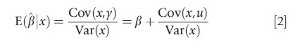
where E is the expectation operator, Cov(x, u) is the covariance between x and u, β is the true value of the causal effect that is to be estimated, and Var(x) is the variance of x. That is, the distribution of the OLS estimator is centered on the causal effect of interest plus a term which depends on the extent to which unobserved causes of the outcome (u) vary with the treatment (x). Here, y may move with x even if x has no causal effect on y, either because y ‘reverse’ causes x, or because x and u share common causes, leading to biased and inconsistent OLS estimates of the causal effect of interest.

The method of IV can solve the problem in some circumstances. Suppose that z is a variable which has the property that z affects y only because z affects x, which in turn affects y, as illustrated in the diagram

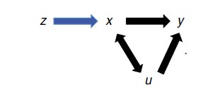
If z affects y only through its effect on x, then correlation between the instrument z and the outcome of interest y implies that x causes y. Under this assumption, the effect of a one unit change in z on y is the product of the effect of z on x and the effect of x on y. The observed association between z and y reveals only the product of these two effects. However, the effect of x on y can be isolated by dividing the observed association between z and y by the observed association of z and x.

The derivation of the IV estimator can be shown more formally (using the method of indirect least squares) as

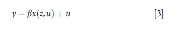
expressing the treatment x as a function of the instrument z and the unobserved causes of y, u. Note that the key condition that z only affects y because z affects x is imposed. Differentiate with respect to z to find

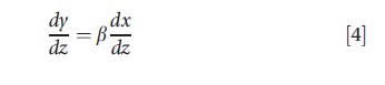
as du/dz = 0 by assumption. Rearrange to find

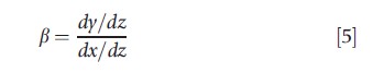
which tells one that the causal effect of interest is the ratio of the effect of z on y to the effect of z on x. If those effects are estimated using linear regressions, then

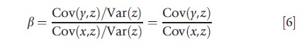
Replacing the population moments in the expression above with sample moments calculated from the data yields the linear IV estimator for this model, denoted β_IV,

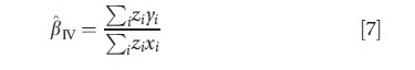
Note that, in contrast to the OLS estimator, the IV estimator depends in no way on the correlation between y and x, which is confounded by the common cause u and therefore does not tell us anything useful about the causal effect of x on y. Note also that, unlike the OLS estimator, the denominator of the expression above is a covariance rather than a variance, and it is therefore not bound away from zero. It is clearly required that Cov(x, z) be different from zero. The problems this issue causes are dealt with below in the discussion on ‘weak’ instruments, which arise when Cov(x, z) is not zero but is small.

General Linear Model And Two-Stage Least-Squares Interpretation

Now consider the general linear problem of estimating causal effects when there are k covariates, an arbitrary number k₁ of the covariates are endogenous (correlated with the error term u), and the remainder k₂ = k–k₁ covariates are exogenous. Let X_1i denote the k₁-vector of observations on endogenous regressors for the ith sampled unit and X_2i the vector of k₂-vector of observations on the exogenous regressors, so that the model to be estimated can be expressed as

It is possible to show that the parameters β₁ and β₂ can be estimated if there are l≥k₁ variables, which are correlated (in a sense defined formally below) with the endogenous regressors X₁ but have no direct effect on y after conditioning on X₂, that is, these variables only affect y because, conditional on X₂, they affect the endogenous regressors X₁. If there are fewer than k₁ such variables, the model is said to be underidentified, and the model is not identified. If there are exactly l = k₁ such variables, the model is said to be exactly identified, and if there are l>k₁ such variables the model is overidentified.

Let Z_i = (Z_1i, X_2i) denote the (l +k₂)-vector of observations for all exogenous variables for the ith unit. Here, Z_1i is the vector of observations on l variables which only affect y because they affect X₁ – these variables do not appear in the equation that is being estimated (eqn [8]), so they are called the excluded instruments. The vector X_2i of observations on exogenous variables in eqn [8] can ‘act as their own instruments.’ The multivariate version of the estimator defined in eqn [6] is

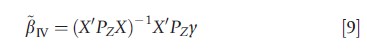
where P_Z= Z(Z`Z)<sup>-1</sup>Z`. It is possible to show that β_IV may be calculated by executing the following steps:

1. Separately for each of the endogenous regressors in X₁, regress the endogenous regressor on the complete set of exogenous variables Z. Save the set of predicted values, X₁.
2. Regress y on X₁ and X₂ using OLS.

The estimated coefficients in step 2 are numerically identical to β defined in eqn [9]. For this reason, the linear IV estimator is sometimes referred to as the ‘two-stage least squares’ (2SLS or TSLS) estimator.

Statistical Properties Of The IV Estimator

In this section, the sampling properties of the IV estimator are briefly described. Formally, the assumptions that the excluded instruments z₁ only (after conditioning on X₂) affect the outcome y through their effect on the endogenous regressors X₁ can be expressed as

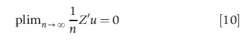
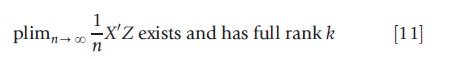
where plim is the probability limit operator as the sample size n tends to infinity. The condition that the excluded instruments must be correlated with the endogenous regressors can be expressed as

Under some further regularity conditions, which is omitted, it is possible to show that

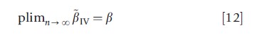
that is, the IV estimator is consistent under these assumptions. If the sample size is allowed to grow arbitrarily large, the difference between the estimates and the causal effects of interest becomes arbitrarily small. Further, the estimator is asymptotically normal, permitting conventional inference with standard test statistics (such as the z-ratios and F-statistics). The covariance matrix can be estimated as s²(X`P_zX)^-1 if the errors u_i are homoskedastic and serially uncorrelated, where s² is a consistent estimate of the variance of u; covariance estimators consistent in the presence of arbitrary heteroskedasticity and serial correlation are also readily available. Finally, the IV estimator is asymptotically efficient in the class of linear estimators.

Note that the IV estimator generally has no desirable small sample properties. It is possible to show that in exactly identified models (models with exactly as many excluded instruments as endogenous regressors),

that is, the estimator has no moments, its distribution has such ‘fat tails’ that the integral defining the expected value of the estimator does not converge. In practice, this means that not uncommonly that one gets ‘wild’ estimates many standard deviations away from the causal effect of interest. Recall that there are k₁ endogenous regressors and l excluded instruments, and that l is required to be at least as large as k₁. The difference (l–k₁) is the number of over-identifying restrictions. It is possible to show that the number of existing moments of β is equal to the number of over-identifying restrictions. For example, if there is one endogenous regressor and one excluded instrument, the model is exactly identified and β does not even have a mean. If one more excluded instrument is added, there is one over-identifying restriction and β has a mean but not a variance nor any higher order moment, and so on.

The IV estimator is generally biased even when at least one over-identifying restriction exists. As the degree of over-identification rises, the bias of the IV estimator rises and approaches the bias of the OLS estimator as the number of over-identifying restrictions approaches the sample size. At the same time, it is possible to show that the dispersion of the IV estimator falls with the number of over-identifying restrictions.

Generally, researchers face a trade-off: The OLS estimator in the presence of endogenous regressors is inconsistent, but is less dispersed than the IV estimator. Which estimator is preferred depends on the trade-off the researcher is willing to make between bias and dispersion. Adding more excluded instruments (and thus increasing the number of over-identifying restrictions) decreases the dispersion of the IV estimator, but increases its bias.

Examples Of Instrumental Variables In Health Research

In this section, some examples of applied IV estimation drawn from the health economics literature are discussed. RCTs are considered as a special case of IV models, and build to more complex models for, first, imperfect RCTs and then uncontrolled experiments.

Example 1: RCT With Perfect Compliance

As a trivial example of IV, consider interpreting standard analysis of an RCT with perfect compliance as an IV estimator. Suppose that y is the outcome of interest, x is a binary variable denoting treatment status such that x_i=1 if subject i is given the new therapy and x_i = 0 if given the standard therapy. The researcher randomly draws a binary variable from a process independent of y (a figurative coin flip); z denotes the outcomes of this process. The researcher then assigns treatment statuses: x_i=z_i. In this scenario, z is determined independently of u, and z is perfectly correlated with x; z thus satisfies the conditions for an IV given above. In this special case, z completely determines x (subjects comply perfectly with their assigned treatment), so that x cannot be correlated with u. As x is exogenous in this case, the IV estimator is the same as the OLS estimator.

Example 2: RCT With Imperfect Compliance

Now consider a common problem with RCTs: suppose some subjects who are assigned to receive the standard therapy nevertheless take the new therapy; others assigned to receive the new therapy actually take the standard therapy. Generally, the difference in sample means across the treatment and control groups reflects both the causal effect of treatment and nonrandom selection into treatment, so it cannot be used to estimate the treatment effect. Assuming that assignment, z, affects the treatment decisions, X, of at least some people, treatment is not randomized because of the noncompliers, but it is quasirandomized in the sense that some of the variation in treatment status is a result of the coin toss. In the case with no other covariates, it is possible to show that the IV estimator defined in eqn [6] takes the form

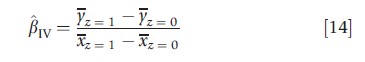
where y_z=i denotes the sample mean of the outcome y in the subpopulation for which the assigned treatment status was i. The numerator is the difference in the average outcome between those assigned to the new therapy and those assigned to receive the standard therapy, regardless of the realized treatment status. This is the key object in ‘intention to treat’ analysis common in the medical literature. The denominator is the difference in the proportion who receive the new therapy across those assigned to new therapy and those assigned to the standard therapy. Note that the denominator is equal to one if compliance is perfect.

Example 3: The Causes Of The Cholera Outbreaks In Victorian Era London

Even if one cannot run an RCT, the real world sometimes provides a mechanism that comes close to the experimental ideal. Perhaps the earliest IV application was that by John Snow, an epidemiologist who was interested in the causes of the cholera outbreaks that afflicted residents of London, England in the 1800s. Snow’s hypothesis, which was not widely accepted at the time, was that cholera is a waterborne pathogen. In particular, Snow suspected that cholera was transmitted via contaminated drinking water. He noticed that one supplier of London’s drinking water provided water contaminated by raw sewage, whereas another supplier provided relatively clean water. The reason was that these suppliers sourced their water from different points along the Thames River, one downstream of the city’s sewer discharge and one upstream. Hence, the first condition for a good IV was satisfied: the identity of water supplier (z) resulted in marked variation in the quality of water consumed by households (x). Moreover, the source of water supply appeared to be independent of u, the other sources of the incidence of cholera. This was important because the quality of the water piped to households, though an important determinant of the quality of water consumed by households (x), was not the only determinant. The level of hygiene and cleanliness also played a role and this varied with household socioeconomic status. However, Snow observed that both the suppliers served a wide cross-section of Londoners, rich and poor alike. Thus Snow’s instrument z was independent of u, the other determinants of y. A comparison of the rates of cholera of households that were supplied by the two water providers provided convincing evidence in support of Snow’s hypothesis.

Example 4: Efficacy Of Healthcare Treatments Without Experimental Randomization

Several studies have compared the effectiveness of different types of healthcare used to treat particular health conditions. Conventional approaches must contend with the possibility that more severely compromised patients may be steered to one treatment over another. IV methods present a way forward when there is a mechanism that causes exogenous variation in the treatment received.

Some analysts have used the ‘differential distance’ to travel to obtain a particular therapy to treat a given health condition. Differential distance is the distance from the patient’s residence to the nearest healthcare facility providing the treatment of interest minus the distance from the patient’s residence to the nearest facility that provides any form of care to treat the condition. The idea is that, particularly for urgent problems such as acute myocardial infarction, the patient receives treatment from the nearest facility, regardless of the illness severity. If the nearest facility happens to provide the treatment of interest (i.e., zero differential distance) then the patient is more likely to receive it. The longer the differential distance, the less likely the patient will receive the treatment of interest. Differential distance is an invalid instrument if particularly ill patients relocate to be close to facilities that provide the treatment of interest.

Other analysts have exploited the marked geographic or interprovider variations in medical practice patterns that appear to be unrelated to medical need or patient preference. These variations were first noted by Glover; he highlighted the striking geographic differences in the rate of tonsillectomy among British school districts. The literature, however, is most closely associated with the small-area variations research of Jack Wennberg. Brookhart, Rassen, and Schneeweiss review the ways in which analysts have used these variations to implement IV estimation of comparative treatment effectiveness. They note that to successfully implement IV, the practice variations must be independent of u, the unmodeled factors that affect patient health outcomes. These include the background characteristics of the patients themselves. It cannot be the case, for instance, that patients with particularly high values of u gravitate toward providers who tend to use the treatment under study. Moreover, practice style must affect health outcomes only through its influence on the treatment under study. Thus, providers who preferentially use one treatment must be of comparable quality and skill to those who preferentially use another treatment.

A third source of exogenous variation is changes over time in the availability of treatments. For instance, a new drug may become approved for use, or, conversely, a drug may be withdrawn from the market for safety reasons. Access to a treatment might also be temporarily impeded. For example, Evans and Lien use the disruption in the availability of public transit due to a bus strike to assess the impact of the use of prenatal care on birth outcomes. They focused on individuals for whom the disruption in bus service would impede access to prenatal care: pregnant black inner-city women. Analyses of this sort require a comparison of outcomes between two periods of time. To implement IV, the expected value of u must be the same in both periods. As Brookhart and colleagues note, to ensure that this condition holds, IVs based on calendar time are most reasonable in situations where a dramatic change in treatments occurs over a relatively short period of time.

Example 5: Effect Of Education On Health

Return to the motivating example in the opening paragraph: To estimate the causal effect of an additional year of education on some measure of health status. Correlations or partial correlations between health and education do not reveal this causal effect because many personal and contextual characteristics (such as intelligence, conscientiousness, and family wealth) affect both health and education and are unobservable to the researcher, and because poor health while young may ‘reverse’ cause poor educational outcomes. That is, the effect of education on health is hard to estimate because of confounding on unobservables and because of ‘reverse’ causation. Neither conventional regression models such as OLS or logit nor matching estimators recover the causal effect of interest, and controlled experimentation on educational outcomes is restricted by both cost and ethical concerns.

In an influential study, UCLA economist Adriana LlerasMuney employed an IV strategy to address this problem. She estimated regressions in which mortality is the health outcome of interest. Using large samples from the US census, she matched cohorts to the number of years of compulsory schooling specific to each combination of state government and year. Years of compulsory schooling acts IV: It is plausible that the only reason a change in years of compulsory schooling affects health is because (for some students) changes in years of compulsory schooling affects realized years of schooling. Intuitively, Lleras-Muney asks, ‘‘Is an adult who was required by law to take more schooling healthier, on average, than a statistically identical adult required to take less schooling?’’ Her estimates suggest that an additional year of schooling causes as much as a 1.7 year increase in life expectancy at the age of 35 years.

Problems With Instrumental Variables Estimation

In theory, it is easy to write down conditions (10) and (11) and derive that an estimator satisfying these conditions can recover causal effects from observational data. In practice, finding variables that satisfy those conditions can be very difficult or impossible. Worse, it turns out that even small deviations from those conditions can yield estimators with extremely poor properties.

The most difficult problem to overcome is instruments which are themselves endogenous, that is, correlated with the error term in the equation of interest, violating condition (10). It is possible to show that the IV estimator is inconsistent when the instruments are endogenous. Intuitively, if our condition that the only reason y varies with z is because z causes x fails, then observing that z and y move together is not evidence that x causes y.

For most problems finding variables that only affect the outcome of interest because they affect the endogenous regressors is challenging. Consider, for example, one of the key problems in the social determinants of health literature: estimating the causal effect of personal income on health. A variable is required which affects health solely through its effect on income. It is unlikely that any personal characteristic satisfies that condition: personal characteristics such as education, smoking status, or cognitive ability all affect income, but all potentially affect health conditional on income, so none are valid instruments. Regional characteristics such as the unemployment rate may affect income, but may also affect health through other channels, such as provision of local public goods or through sorting of people across states. Researchers therefore need to be creative in finding valid instruments: one study, for instance, uses lottery winnings as an exogenous source of income to assess the effect of income on the health of lottery players. In other applications, valid instruments may simply not be available.

It may seem that variables which are almost, but not quite, exogenous may yield reasonable estimates, provided that there is a large sample and can thus rely on the consistency property of the IV estimator. In particular, from the formula for the probability limit of the univariate IV estimator presented above, it is possible to show

As long as Cov(z, u) is close to zero, then the ratio of Cov(z, u) to Cov(z, x) should itself be close to zero. This intuition is correct provided that Cov(z, x) is sufficiently large. If, however, there is only weak correlation between z and x then even small violations of exogeneity lead to very poorly behaved estimates. The reason is that Cov(z, u) is divided by a number close to zero, which has the effect of amplifying Cov(z, u). The result is that the IV estimator β_IV can be centered on a value wildly different from the true value of β, even as the sample size grows arbitrarily large. A low level of correlation between the instruments and treatment is known as the ‘weak instrument problem.’

What is more, even if the instruments are exogenous, if the instruments are weak the IV estimator will tend to be badly biased in finite samples and, perhaps worse, the usual estimator of the covariance matrix, and test statistics based on that matrix, will be biased, leading to severe size and power distortions. The bias stems from the fact that the IV estimator is the ratio of two estimators – the numerator being the estimator of the effect of z on y and the denominator the estimator of the effect of z on x. In large samples, these estimators converge to their population quantities. In finite samples, however, sampling error in the two estimators can cause the ratio to behave erratically. The weaker the instruments, the greater is the sampling error.

In short, instruments with poor properties – either endogenous or weak – may be ‘cures worse than the disease.’ The good news is that in overidentified models it is possible to construct test statistics against the null that the instruments are exogenous, and it is always possible to test the strength of the instruments.

Heterogeneous Causal Effects

Over the past two decades the IV literature has focused on the following issue: If different entities or ‘units’ (people, firms, hospitals, etc.) experience different causal effects as a result of the same treatment, how are we to interpret IV estimates? It turns out that when treatment effects are heterogeneous, identification of causal effects using IV can be challenging.

Consider a slight modification to eqn [1],

which differs from eqn [1] only in that the slope coefficient β_i may vary arbitrarily across units. In the interest of simplicity, again suppose x_i is a binary indicator of whether unit i received treatment.

In this model, it is incoherent to refer to ‘the’ causal effect of x on y, as each unit generally experiences a different causal effect. Estimation of counterfactual outcomes in this model is also more complicated than in model (1). When treatment effects are constant, the outcomes of untreated units can be used to infer the counterfactual outcomes of those that were treated (and vice versa). This is not generally possible when causal effects vary across i. Therefore it is not possible to estimate the effect of treatment for any given unit. Researchers instead attempt to estimate features of the distribution of the causal effect, bi, such as the population average treatment effect, E(β_i), or the average treatment effect for those who actually received the treatment, E(β_i| x_i = 1).

Without loss of generality, write β_i = β+ε_i, where β is the population mean effect and ei is a zero-mean idiosyncratic effect specific to unit i. Substituting into eqn [16],

Notice that the error term contains two components: unobserved causes of the outcome specific to unit i, μ_i, and the interaction between treatment status and unit i’s return to treatment. If both mi and ε_i are uncorrelated with x_i, OLS estimation is consistent for the average treatment effect, β. However, even when μ_i is uncorrelated with x_i, correlation between ε_i and treatment status creates an endogeneity problem and OLS does not recover the average treatment effect. In this case, ‘essential heterogeneity’ is said to exist. Essential heterogeneity commonly occurs in observational studies of treatment efficacy when individuals with the most to gain from taking a particular treatment are more likely to receive that treatment. Essential heterogeneity can also exist in RCTs with imperfect compliance. This occurs if subjects are able to: (1) determine the treatment to which they have been assigned, (2) predict better than chance which treatment will benefit them most, and (3) if advantageous, switch therapies. Condition (1) occurs if subjects are not blinded or if they are blinded, subjects can infer treatment status from side effects, or other physiological clues. The extent to which condition (3) holds depends on the context. Subjects assigned to the new therapy who wish to use the standard therapy can presumably obtain the standard therapy outside the trial. Conversely, subjects assigned to the standard therapy who wish to use the new therapy might be able to obtain the new therapy from friends enrolled in the trial.

Estimation using IV is complicated by essential heterogeneity. The instrument must be correlated with treatment status: It must move some people into or out of treatment. Even if all of the conditions defined in section The Instrumental Variables Estimator hold, the properties of the IV estimator depend on which people get moved into or out of treatment when treatment effects vary across people. Consider again example 2 in section The Instrumental Variables Estimator above, an RCT with imperfect compliance. Under a condition called monotonicity, which requires that there be no ‘defiers’ – people who only receive treatment if they are assigned not to receive treatment or vice versa – it is possible to show that the IV estimator converges to the average causal effect of treatment of compliers, that is, subjects who use the treatment that they were assigned to. This is called the ‘local average treatment effect’ arising from this treatment.

Intuitively, some people will always take the new treatment and others will always take the standard treatment, regardless of the assignment. The experiment does not change these people’s behavior and therefore the experiment generates no information about the causal effects of treatment for these people. The IV estimator depends solely on the outcomes of subjects whose treatment status was experimentally manipulated; the estimator tells us the average effect only for that (unobservable) subpopulation. If the instrument takes many values instead of just two, it is possible to show that (under monotonicity) the IV estimator converges to a difficult-to-interpret weighted average of local treatment effects, in which units for which treatment status is most responsive to variation in the instruments receive the highest weights.

In addition to complicating the interpretation of conventional IV estimates, heterogeneous causal effects complicate specification testing. Most tests of the assumption that the instruments are exogenous are based on stability of the estimates as different sets of instruments are used to construct the estimator. Under homogeneous responses, all of these estimates converge to the causal effect. When effects are heterogeneous, different instruments recover different weighted averages of local effects, and will differ even if the classical conditions (10) and (11) hold, so rejection of the null can no longer be interpreted as evidence that the instruments are endogenous.

Example: Reinterpreting An Estimate Of The Effect Of Education On Health

Consider again example 5, above, of research using IV on the effect of education on health. Earlier, Lleras-Muney’s estimates were interpreted as suggesting that an additional year of education causes an increase in life expectancy of 1.7 years at the age of 35 years. Lleras-Muney’s estimates are based on variation in compulsory schooling laws, so she interprets her IV estimates as: among the subpopulation who only receive additional education if and only if they are forced to do so by law, an additional year of education increases life expectancy by 1.7 years at the age of 35 years. This subpopulation may experience substantially different health returns to education than other people who choose to go on to receive more than the legally mandated minimum schooling. Thus, LlerasMuney’s local average effect may not reflect the health returns to education for other groups. However, Lleras-Muney’s estimates may be more relevant than results from a hypothetical RCT randomizing education if policy questions hinge on effects experienced by people whose educational outcomes are affected by changes in compulsory schooling laws, as the RCT would recover population average effects rather than effects for the subpopulation affected by policy changes.

References:

1. Brookhart, M. A., Rassen, J. A. and Schneeweiss, S. (2010). Instrumental variable methods in comparative safety and effectiveness research. Pharmacoepidemiology and Drug Safety 19(6), 537–554.
2. Brooks, J., Irwin, C., Hunsicker, L., et al. (2006). Effect of dialysis center profitstatus on patient survival: A comparison of risk adjustment and instrumental variable approaches. Health Services Research 41, 2267–2289.
3. Evans, W. and Lien, D. (2005). The benefits of prenatal care: Evidence from the PAT bus strike. Journal of Econometrics 125, 207–239.
4. Glover, J. (1938). The incidence of tonsillectomy in school children. Proceedings of the Royal Society of Medicine 31, 1219–1236.
5. Heckman, J. J., Urzua, S. and Vytlacil, E. (2006). Understanding instrumental variables in models with essential heterogeneity. Review of Economics and Statistics 88, 389–432.
6. Jones, A. (2009). Panel data methods and applications to health economics. In Mills, T. and Patterson, K. (eds.) Palgrave handbook of econometrics, vol. 2, pp. 557–631. London: Palgrave MacMillan.
7. Jones, A. and Rice, N. (2011). Econometric evaluation of health policies. In Glied, S. and Smith, P. (eds.) Oxford handbook of health economics, vol. 1, pp. 890–923. Oxford: Oxford University Press.
8. Lleras-Muney, A. (2005). The relationship between education and adult mortality in the United States. Review of Economic Studies 72(1), 189–221.
9. McClellan, M., McNeil, B. and Newhouse, J. (1994). Does more intensive treatment of acute myocardial infarction in the elderly reduce mortality? Analysis using instrumental variables. Journal of the American Medical Association 272, 859–866.
10. McConnell, K., Newgard, C., Mullins, R., Arthur, M. and Hedges, J. (2005). Mortality benefit of transfer to level I versus level II trauma centers for headinjured patients. Health Services Research 40, 435–457.
11. Pop-Eleches, C. (2006). The impact of an abortion ban on socioeconomic outcomes of children: Evidence from Romania. Journal of Political Economy 114, 744–773.
12. Stock, J. H., Wright, J. H. and Yogo, M. (2002). A survey of weak instruments and weak identification in generalized method of moments. Journal of Business & Economic Statistics 20(4), 518–529.
13. Tan, H., Norton, E., Ye, Z., et al. (2012). Long-term survival following partial vs radical nephrectomy among older patients with early-stage kidney cancer. Journal of the American Medical Association 307, 1629–1635.
14. Wennberg, J. (2008). Commentary: A debt of gratitude to J. Alison Glover. International Journal of Epidemiology 37, 26–29.
15. Xian, Y., Holloway, R., Chan, P., et al. (2011). Association between stroke center hospitalization for acute ischemic stroke and mortality. Journal of the American Medical Association 305, 373–380.