Evaluating Efficiency of a Health Care System

Introduction

The way economists look at the production of health care is to examine the relationship between the inputs into and the outputs from a production process as illustrated in Figure 1.

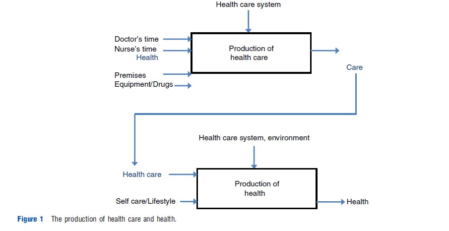
Figure 1 is a flow diagram showing how inputs such as medical staff and equipment produce health care, for example, the services offered by a hospital, and how use of these type of available health care inputs are converted into actual health itself, for example, curing a disease. Health itself, of course, is influenced by matters other than the health care system – such as housing conditions, education levels etc., which are often also accounted for in such models of how health is produced. Economists are interested in how one can make these production flows as resource efficient as possible because health care is very expensive, on average using up over 10% of developed countries GDP. To do this, the most efficient use of the inputs to these processes to produce the desired output is looked at – in most cases, to maximize health. In the top half of Figure 1, one can see how health care is produced given certain inputs, such as medical staff time. In the bottom half of Figure 1, health care becomes an input to a person’s health, along with all the other things outside the health care system that contribute to health itself.

Mostly, research in this area has concentrated on the top half of Figure 1, as the inputs to, and the outputs from a health care organization can be measured, for example, a hospital. So, what sort of things would be inputs and outputs to the production of health care? It can be thought about in terms of a hospital, the most recognizable unit of health care production in a developed country, and the largest consumer of resources. Inputs include things like doctors and nurses, equipment and drugs, and capital, such as buildings and beds. Outputs are produced by the hospital – so, for example, numbers of patients treated – ideally adjusted in some way for the quality of care they produce – numbers of different operations undertaken, or diagnostic tests.

This article will describe how the relationship between inputs and outputs can be measured, and how information that improves the efficiency of how these services are delivered can be provided – the benefit being an improvement in the efficiency of production of service delivery and ultimately the production of patient health. It begins with a discussion of alternative techniques for measuring efficiency. Theoretical foundations are based on the pioneering work of Farrell (1957).

Two alternative approaches to measuring efficiency of a health care system are described: data envelopment analysis (DEA), and stochastic frontier analysis (SFA). The article then describes how best to make use of techniques such as these in terms of a system of protocols and gives guidelines for how to provide the most appropriate information to those involved in policy making and service delivery.

Efficiency Measurement

In economic terms technically efficient combinations of inputs are those which use the least resources to produce a given level of output (for a given state of technology). Alternatively, technical efficiency (TE) may be defined in terms of maximizing output for a given level of inputs. By contrast, full allocative efficiency is achieved by selecting combinations of inputs (e.g., mixes of labor and capital) which produce a given amount of output at minimum cost (given market prices for inputs), i.e., there can be no improvement in output by simply reallocating resources. The first measure looks at physical quantities, the second introduces a cost element.

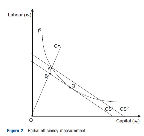
Farrell’s seminal work introduced two further concepts: radial measures of efficiency; and overall (economic) efficiency. These concepts are illustrated in Figure 2. The figure considers a simple example of producing a single aggregated output ‘health care’ from two inputs: medical labor (x₁) and capital (an example often used is beds)(x₂), The parallel lines (CS¹ and CS²) represent isocost lines (which show relative input combinations that cost the same) and I°, an isoquant (simply a line drawn through a combination of input points used to produce the same level of output). Assuming a hospital chooses a desired health care output level y°, to be technically efficient they should choose a combination of inputs which lie on I°. Producing quantity y° using inputs at point C would be technically inefficient because the hospital could produce y° using both less labor and beds. Keeping the same mix of inputs, a hospital would be technically efficient if they are produced at point A, which lies on the isoquant. Farrell’s measure of TE is based on the line OC, which passes through A and C. OC is often referred to as a radial measure of efficiency as it measures efficiency in terms of distance from the origin. TE at point C is given by the radial measure:

where TE must take a value greater than zero and less than or equal to one (0<TE≤1). If TE = 1, the hospital is technically efficient and is operating on the isoquant. If TE<1 the hospital is technically inefficient.

If a hospital wishes to minimize costs, they will choose the combination of labor and beds at point Q where the isocost line CS₁ is tangential to I°, and where the combinations of inputs cost the least to produce the given level of output. If the hospital chooses an input mix (e.g., they may be legally obliged to have a certain number of doctors employed to offer certain services) along the line OC and is technically efficient they will produce at point A, which, lies on the isocost line CS₂. However, this implies they are not minimizing costs. The allocative inefficiency of choosing the input mix at point A (which is technically efficient) can be captured as the ratio of the costs of producing at A compared to the costs of producing at the allocative efficiency level, point Q, where the latter costs are given by the icocost line CS₁ (the ray OA intersects this isocost line at B). This is the ratio:

where similarly AE must take a value greater than zero and less than or equal to one (0<AE≤1). When AE is less than 1 this implies that production is not allocatively efficient. AE can be interpreted as a measure of excess costs arising from using inputs in inappropriate proportions. If producing at 0Q the hospital would be technically and allocatively efficient, otherwise, if, for instance, a particular input mix is imposed on the hospital, it can achieve TE but not necessarily allocative efficiency.

Farrell’s TE and AE terms can be combined to generate a measure of overall (economic) efficiency (OE) for production at point C:

where OE also lies in the range (0<OE≤1).

Empirical measurement of these concepts can now be considered.

Data Envelopment Analysis

DEA is by far the most common method for analyzing efficiency in health care. It has now been applied over 400 times in health care settings. DEA is a mathematical technique which makes use of linear programming methods. It is based on the idea of efficiency as the relationship between the outputs from an activity and the amount of inputs that the activity uses. In the simple case of a single output/single input firm a measure of TE can be defined as:

where y = output and x = input.

The greater this ratio, the greater the quantity of output for a certain amount of input, as measured in natural (noncost) units. For a multiple-output/multiple-input firm, like a hospital which treats different types of cases using staff of different types, various equipment and so on, an overall measure of a hospital’s TE is:

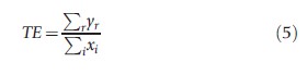
where i is input, and r is output.

The problem with this is that inputs and outputs cannot be simply summed as they usually measure very different things, for example, numbers of doctors, and numbers of operating theaters). Rather, weights to each of the inputs and outputs are given so that:

where: y_r = quantity of output r; u_r = weight attached to output r; x_i = quantity of input i; v_i = weight attached to input i; and p and m are the numbers of outputs and inputs. As is explained below, the weights are chosen so that 0<TE≤1. Thus, DEA is founded on an indicator of efficiency which can be calculated for each firm and, if u and v are fully flexible, is defined as the ratio of a weighted sum of the outputs relative to a weighted sum of its inputs.

The efficiency of any firm or unit, say a hospital (or nursing home, GP practice etc.), can be measured relative to other units within a peer group. Because the weights are unknown a priori, they must be calculated. Of all of the possible sets of weights which would satisfy all of the constraints, the linear program optimizes the ones that give the most favorable view of the unit. This is the highest efficiency score, the one that shows the hospital in the best possible light. This problem can be expressed as a fractional program. Such programs are difficult to solve, but can be reformulated into a straightforward linear program (LP) by constraining the numerator or denominator of the efficiency ratio to be equal to unity. This recognizes that in maximizing a ratio it is the relative values of the numerator and denominator that are important, not their absolute values. The problem then becomes to either maximize weighted output with weighted input equal to unity, or minimize weighted input with weighted output equal to unity. The output-maximizing LP is:

For h₀ in a sample of n hospitals,

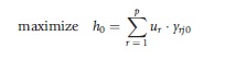
subject to:

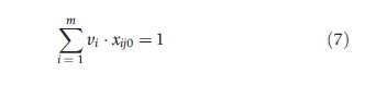
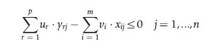
where: h₀ is the measure of relative TE of hospital 0, j is the References: set of 1…n hospitals, and e is an infinitesimal.

In eqn [7], the denominator (weighted inputs) has been set equal to unity and the numerator (weighted outputs) is being maximized. One model must be solved for each hospital in the sample in turn, and can be solved using standard LP methods to give an efficiency score for each hospital.

The minimization rather than the maximization of this LP is simpler to solve and has a useful interpretation. If one now calls h₀ Z₀ to represent the opposite (or dual) measurement one is taking in a sample of n hospitals,

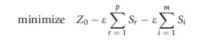
subject to

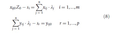
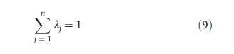
where: λ_j, s_r, s_i≥ 0 j, i and r; λ_j are weights on units, sought to form a composite hospital to outperform j_o; s_i are the input slacks; and, s_r are the output slacks.

Essentially, the dual finds a set of weights for each hospital which minimizes an inefficiency measure subject to constraints. The hospital will be efficient if s_i = s_r = 0 and Z_o = 1, that is, a composite hospital cannot be constructed which outperforms it. This is the best that can be achieved in production terms using the combinations the hospital has available to it. If Z_o <1 and/or s_i >0, s_r >0, the hospital will be inefficient. The composite hospital provides targets for the inefficient hospital and Z_o represents the maximum inputs a hospital should be using to attain at least its current output. The weighted combination of inputs over outputs for each hospital forms the production frontier. The hospitals which lie on this frontier, that is those which have a TE score of one using the weights of a References: unit, are called the ‘peers’ of the References: hospital.

DEA uses the assumption of either constant or variable returns to scale (CRS or VRS). The LP in eqn [7] or eqn [8] calculates the CRS production frontier. A VRS frontier is obtained by adding a further constraint to the dual of the LP:

The extra constraint requires more units. Because the production function is not directly observable, DEA estimates a production frontier based on input and output data. The frontier maps the least resource use input combinations and is assumed to be convex to the origin. The DEA frontier is illustrated in Figure 3 and (like Figure 2) considers a simple, single output, two input example. The dots represent different producers and the quantities of inputs they use to produce the same given level of output. The DEA frontier (I1I0) consists of straight lines joining the points that represent the most efficient producers. Inefficient producers lie to the right of the frontier. The complete production frontier covering all levels of output can be inferred, and the analysis can be extended to cover both multiple inputs and outputs, and the assumption of CRS can be dropped.

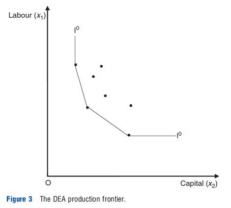
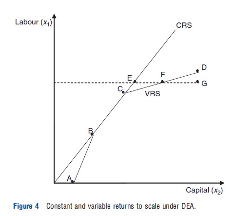
Figure 4 illustrates DEA frontiers under CRS and under VRS. The frontier is drawn slightly differently to Figure 3 to introduce how the concepts VRS and CRS are important in DEA. The section AB of the VRS frontier exhibits increasing returns to scale (output increases proportionately more than inputs), BC exhibits CRS, and CD decreasing returns to scale (output changes proportionately less than the change in inputs). For a given hospital, G, the distance EF measures the effects of economies of scale in production, and FG measures ‘pure’ inefficiency. Clearly, more hospitals will be deemed to be efficient under variable returns to scale, as under an assumption of CRS any economies of scale are included in the measure of inefficiency.

DEA (in the formulation presented above) does not account for the influences of the distribution of medical case complexity (casemix) on producer efficiency in the production of health care. One approach to modeling the effects of casemix is to include the patient characteristics (for patients at different health care hospitals) as a type of input in the production frontier. However, this approach may be inconsistent with economic theory, as patients are not inputs which are transformed to make the final product (which in this case is a health care intervention). Instead, patients consume treatments to (hopefully) produce improvements in their health status.

The characteristics of patients and their illness will influence the production of health care in order to produce these health status improvements, hence patient illness differences (e.g., the intensity of a heart attack, or the stage of a cancer) may be better viewed as factors which shape the outputs rather than inputs in the production process. DEA models can incorporate this approach to patient illness characteristics (casemix factors) by modeling the effect of casemix on the overall production process by adjusting outputs by casemix group. Another method involves adding a second stage of analysis to the DEA approach. The first stage of the model involves running a DEA model based on physical inputs and treatment-based outputs to yield efficiency scores for units (say hospitals again), as shown above. The second stage then takes these efficiency scores and regresses them against hospital level casemix variables to assess the impact of the patients’ socio-demographic and clinical characteristics on the production process and efficiency. This allows the inclusion of variables which do not fall neatly into the input–output analysis and potentially see if they have a significant impact on the efficiency scores obtained in the first stage, but there are many statistical issues with undertaking such second stage analysis (Fried et al., 2008).

Some Limitations

Before proceeding, it is important to note that DEA has several major limitations which require some care on the part of those constructing models and others interpreting the results. There are major statistical issues to account for. The technique is deterministic and outlying observations can be important in determining the frontier (made up of the most efficient units). Closer investigation of these outliers is often warranted to ensure the sample is actually uniform in nature, i.e., one really is comparing like with like. Care must be taken in interpreting results as the DEA frontier may have been influenced by stochastic variation, measurement error, or unobserved heterogeneity in the data. DEA makes the strong and nontestable assumption of no measurement error or random variation in output. Small random variation for inefficient hospitals will affect the magnitude of the inefficiency estimate for that hospital. Larger random variation may move the frontier itself, thereby affecting efficiency estimates for a range of hospitals.

DEA is sensitive to the number of input and output variables used in the analysis. Overestimates of efficiency scores can occur if the number of units relative to the number of variables used is small. A general rule of thumb is that the number of units used should be at least three times the combined number of input and output variables.

DEA only provides a measure of relative efficiency in the sense that: a hospital which is deemed efficient using DEA is only efficient given the observed practices in the sample which is being analyzed. Therefore, it is possible that greater efficiency than that observed could be achieved in the sample.

The Malmquist Index

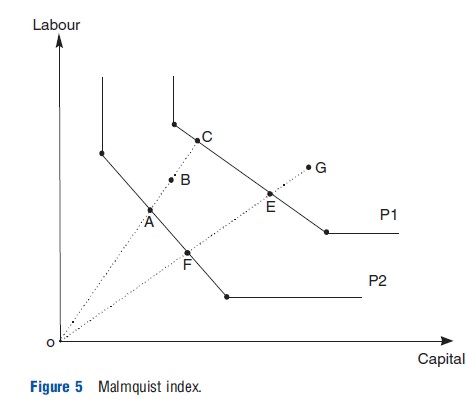
Efficiency can change over time, and DEA based Malmquist indices (named after a pioneering researcher in this area) reused to measure this concept of productivity. The Malmquist productivity index (Fried et al., 2008) is defined as (with References: to Figure 5, a two input, one output model, two time period, where G and B represent a hospital in two different time periods):

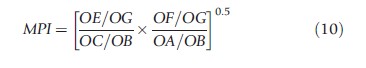
The index is the geometric mean of two indices. In the first the production frontier of period 1 (P1) is taken as given and measures the distance of the two production points, G and B, from it. The second index is similar except the References: frontier is that of period 2 (P2). A score greater than unity indicates productivity progress as a hospital delivers a unit of output in period 2 using less inputs. In other words, the hospital in period 2 is more efficient relative to itself in period 1. Similarly, a score less than unity implies productivity regress and constant productivity is signaled by a unit score. The index can be decomposed:

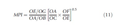
The component outside the brackets is the ratio of TE in each period and measures efficiency change when moving from period 1 to period 2. It indicates whether the hospital gets closer to its production frontier, i.e., becomes more efficient (with a score greater than unity), or moves further away from the frontier, i.e., becomes less efficient (with a score of less than unity), or stays the same (with a unit score). The second component of the Malmquist index in eqn [10] captures technological change evaluated from both time periods, i.e. movements of the actual frontier itself – the technology with References: to which a sample operates. The frontier (i.e., technology) can progress (with a score greater than unity), regress (with a score of less than unity), or stay in the same position (with a unit score). Malmquist indices are increasingly used in health care.

Stochastic Frontier Analysis

SFA, see Coelli et al. (2005) has been used in a much smaller number of efficiency analyses in health care than DEA, but the number of papers is increasing. SFA on cross sectional data decomposes a regression error term into two parts. Given a model of the form:

where y_i is the vector of outputs, xi is the vector of inputs, b is the vector of parameters (of little interest in the context of these models) u_i is the one sided inefficiency term (u_i≥ 0 for all i), vi is the two sided error term which is assumed to follow the usual classical linear regression model error term, and u_i and v_i have zero covariance. Note i,u,x,v all are now discussed with separate and new meanings to the equations in the DEA models above.

The first of the two error terms is a one-sided ‘error’ term that acts as a measure of inefficiency. By constraining this term to be one-sided, production units can only produce on or below the estimated production frontier. The second part is the ‘pure error’ term that captures random noise, and has a two sided distribution. The one sided constraint on the distribution of the inefficiency term allows a realized production frontier to be estimated, and each producer’s efficiency to be measured relative to that frontier.

The use of SFA in the production of health care has received increasing attention over recent years. This is partly because of increased interest in efficiency measurement in general in health and health care, as discussed earlier, as discussed earlier but also because of advances in modeling techniques and increased computing capabilities.

To allow multiple outputs to be modeled (as outputs in health care are typically heterogeneous) researchers often estimate cost rather than production frontiers. Estimation of an SFA production frontier requires that all outputs can be meaningfully aggregated into a single measure. This assumption is questionable in the health context. However, costs can be easily aggregated into a single measure using monetary units such as dollars. The estimation of the cost frontier remains a valid method for examining productive efficiency as it is the dual of the production function. The cost frontier formulation of the model is:

where c_i is expenditure at hospital i, p_i is a vector of input prices, and z_i is a vector of producer characteristics which includes casemix variables. The inclusion of variables capturing casemix and producer characteristics in the model allows statistical testing of hypotheses concerning the relationship between these factors and producer efficiency.

The stochastic frontier model is estimated by maximum likelihood and requires that the researcher specifies an appropriate distribution for the inefficiency term. The most commonly adopted approach for cross-sectional data is to assume that u_i follows a half-normal distribution:

and

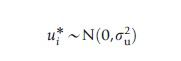
Other distributions suggested for cross-sectional data include the exponential and gamma distributions. However, there are no strong a priori theoretical reasons for choosing any of the above distributions over each other. It has been argued that this has led to arbitrary and nontestable assumptions about the distribution of the inefficiency term, which are a potential source of model misspecification. Another approach adopted has been to use panel data which has the advantage that it requires no specific assumption about the distribution of u_i (Fried et al., 2008).

Assumptions concerning the error term vi in SFA may also be important. If the assumption of normality in the error term does not hold, and its distribution is skewed, inefficiency may be under or over estimated (Jacobs et al., 2006). Because the error term vi is assumed to show zero skewness, any skewness is attributed to the inefficiency term u_i. For instance, periodic capital repairs to a hospital may lead to a positive skew in total cost and hence in the error term. Under a stochastic cost frontier model this will result in inefficiency being detected, even if the hospitals studied are perfectly efficient. Conversely, a negative skew on the error term will bias the estimate of inefficiency downwards. Further, SFA may also reject the null hypothesis of no inefficiency too readily.

The SFA cost frontier is often estimated using a generalized functional form known as a ‘translog’ function, which allows the testing of a wide range of assumptions about the nature of the cost function, and does not impose restrictive a priori assumptions on its functional form. Translog multiproduct cost functions can also be used easily to test for the presence of economies of scale and scope. However, this approach requires a large number of degrees of freedom. In hospital studies, where sample sizes are often small, this may introduce measurement error and bias in inefficiency estimates through the inappropriate aggregation of inputs and outputs. An alternative approach is to impose a functional form which is less demanding on the data (e.g., Cobb-Douglas), but this may come at the price of introducing misspecification into the model.

Making Best Use Of Efficiency Measures In Health Care

It has been postulated that efficiency measurement studies in health care are being produced at an increasing rate, but there is a limited amount of use of such studies in practical terms. Criteria have been suggested previously for assessing the use and usefulness of such studies, from the perspective of the supplier of such studies, and those who might make use of them (Hollingsworth, 2012).

Use And Usefulness Criteria For Suppliers And Demanders

Suppliers

1. Applied research needs to be placed in a policy context. One important element of any efficiency analyses is to get potential end users involved early on. This helps ‘ownership’ of the research from the users’ perspective, and keeps the researcher on track. This may initially involve finding the right person, or group of people (having a number of people involved reduces risks, e.g., staff moving positions). Meetings to feedback results at various stages, and to different levels of users, for example, hospital managers, health department staff, will help make sure information is provided to those who want to use it. An advisory group to initially help set up model specification may be useful.
2. Hospital managers may have concerns about health authorities using efficiency measures as ‘big sticks’ and are generally interested in more detailed information on their specific unit, whereas health authority staff tend to be more interested in the overall picture and comparisons between hospitals. The researcher has to balance these views and providing all the information to everyone may help. One should also ask what information it would be useful to provide that the data/ modeling is not providing right now, and try and accommodate this, or suggest means (e.g., extra data) which could help.
3. Hase the objective of giving end users the information been met? Surveying them, perhaps including a short report, may help refine the measures. Disseminate the results as widely as possible. Make sure users know the limitations of efficiency measures, and that they are a useful policy tool, not the useful policy tool. Results can be manipulated so full provision of information to all may be helpful.
4. Are the right questions being asked?
5. What is the underlying economic theory of production (or cost, does duality theory and the requirement for cost minimization as an objective really apply)?
6. Is the model specified correctly? Hasan extensive sensitivity analysis been undertaken? Ask the advisory group if there are any obvious omitted variables.
7. Are the data really good enough to answer the questions, particularly the output data?
8. Is there any data on quality of care? What will results using just quantity (throughput) data really show? Will any inefficiency be just made up of omitted quality data?
9. If quality data is available, how will it be weighed relative to quantity data, to avoid it being ‘swamped’ by relatively large numbers of throughput information? Unless carefully weighted, potentially vital information on quality may have little impact on results.
10. Is the sample inclusive enough, and is one comparing like with like? Exploratory analyses are useful. Just because all hospitals in the sample have the sample categorization, there may be a rogue specialist unit or teaching hospital that may confound the results. Frontier techniques are very susceptible to outliers. Sample size is also an issue.
11. If one is happy with the data and models, what techniques will be used, DEA, SFA or both? If there are multiple inputs/outputs, nonparametric techniques have an advantage (when comparing DEA and SFA) in terms of disaggregation (Coelli et al., 2005). They allow one to feedback more detailed information on areas of inefficiency. Panel data techniques will also allow one to feedback more information, not only on what happens between units, but also what happens over time. Looking at trends over time is more useful than a snap shot.
12. Is two stage analyses being undertaken, if so how are any statistical problems being accounted for?
13. Does one need to generate confidence intervals? Unless one is certain that the sample is all inclusive, then one might wish to account for sampling variation.

Demanders

Table 1 presents a checklist for assessing if an efficiency analysis should be judged as potentially useful. This (again) is a starting point, based on the Drummond et al. (2005) list for assessing economic evaluations. Suppliers of efficiency studies may also wish to take note of these points. The following two assessment questions asked by Drummond et al. (2005) are also pertinent here: Is the methodology appropriate and are the results valid; and if the answer to this is yes, then – do the results apply in this setting? As Drummond et al. (2005) acknowledge, it is unlikely every study can fulfill every criteria, but criteria are useful as screening devices to identify strengths and weaknesses of studies, and of course to identify the value added by comprehensive extra analysis of this nature.

Summary

The number of studies which seek to measure health service efficiency and productivity continues to increase quite dramatically. Research in this area should be reviewed carefully and the results of studies interpreted and used cautiously, as it is still an area under development. Estimated results can be sensitive to changes in the basic assumptions and specifications of the models used, and the characteristics of the environment in which the units operate. Thus, as concluded previously, the results may only be valid for the units under investigation raising generalizability issues.

A number of criteria are suggested for judging whether research published in this area is potentially useful in a policy context. It should be noted that, as with the original economic evaluation criteria on which they are modeled, these criteria should be used as a means to interpret results, not a checklist for dismissing the usefulness of individual studies on a generic basis. What is of no use to one user may be very useful to another, working from a different viewpoint in a different health system.

In terms of ‘best practice’ for undertaking efficiency studies, it may be that the use of multiple techniques might help indicate trends in inefficiency. If the multiple techniques (parametric and nonparametric, including techniques which can account for multiple objectives) point to the same inefficient organizations, and the organizations cannot sensibly explain them away (i.e., omitted variables and policy shocks), then perhaps some form of inefficiency is being picked up. Of course it may be that in certain circumstances one method is obviously more useful: for example, when there are multiple outputs, SFA may not be appropriate because of problems with having to aggregate variables. Justification of the method used is sometimes difficult at present as there are few criteria for which is ‘best,’ although in practice different measurement methods often show similar results. Another danger at present is relying on exact numbers: small differences in inefficiency may not truly reflect inefficiency, and should be viewed with caution. Trends over time may be more reliable.

As economists the basics of what is meant by efficiency should be kept in mind. However, not only must one decide how efficiency and productivity is measured (efficiency changes over time in the context here), but also why, and how important it is relative to other societal objectives in terms of the delivery of health care. These are all questions left to be answered in a research context.

References:

1. Coelli, T., Rao, D. S. P., O’Donnell, C. J. and Battesse, G. (2005). An introduction to efficiency and productivity measurement. New York: Springer.
2. Drummond, M., Sculpher, M., Torrance, G., O’Brien, B. and Stoddart, G. (2005). Methods for the economic evaluation of health care programmes. Oxford, UK: Oxford University Press.
3. Farrell, M. J. (1957). The measurement of productive efficiency. Journal of the Royal Statistical Society: Series A 120(3), 253–281.
4. Fried, H., Lovell, C. and Schmidt, S. (2008). The measurement of productive efficiency and productivity growth. New York: Oxford University Press.
5. Hollingsworth, B. (2012). Revolution, evolution, or status quo? Guidelines for efficiency measurement in health care. Journal of Productivity Analysis 37(1), 1–5.
6. Jacobs, R., Smith, P. C. and Street, A. (2006). Measuring efficiency in health care. Cambridge, UK: Cambridge University Press.
7. Hollingsworth, B. (2003). Non-parametric and parametric applications measuring efficiency in health care. Health Care Management Science 6(4), 203–218.
8. Hollingsworth, B. (2008). The measurement of efficiency and productivity of health care delivery. Health Economics 17(10), 1107–1128.
9. Hollingsworth, B., Dawson, P. and Maniadakis, N. (1999). Efficiency measurement of health care: A review of non-parametric methods and applications. Health Care Management Science 2(3), 161–172.
10. Hollingsworth, B. and Peacock, S. (2008). Efficiency measurement in health and health care. UK: Routledge.