Statistical Issues in Economic Evaluations

Introduction

As health economic evaluation has become increasingly popular, so it has become much more common that individual patient data are collected alongside clinical trials. This has opened up the possibility of using statistical methods to analyze health economic data with the purposes of informing health economic evaluation.

In this article, statistical methods for analyzing health economic data are reviewed. The second section focuses specifically on issues relating to the analysis and testing of cost data, including issues related to nonnormality of the data, censoring of cost-data and other forms of missingness. The third section deals with characterizing uncertainty in cost-effectiveness (CE) analysis, focusing on the commonly employed incremental CE ratio statistic. The fourth section focuses on the net-benefit statistic as an alternative approach to characterizing uncertainty in CE analyses. A final section offers some concluding comments and links to other articles that address similar material, in particular the increasing use of individual data analyses within CE modeling to address issues of heterogeneity in CE.

Analyzing Individual-Level Cost Data

Where health care resource information has been collected alongside randomized controlled trials, so the formal statistical testing of cost differences has become possible. Nevertheless, a number of problems plague cost data in particular. First, that cost data are often highly nonnormal, exhibiting excess zeros, skewness, and kurtosis. Second, that censoring of cost occurs, just as it does for other trial endpoints. Third, that cost data are often missing, due to the nature of the data collection process.

Non Normality

It is well recognized that statistical analysis of healthcare resource use and cost data poses a number of difficulties related to the distribution of these data: they often exhibit substantial positive skewness, can have heavy tails and often have excess zeros representing a proportion of subjects that are not users of health care resources. In medical statistics, the standard approach for handling such nonnormal data has been to use nonparametric methods, such as rank order statistics. However, in health economics it is widely accepted that it is the estimated population mean cost that is the statistic of interest to policy makers – as only the mean cost (when multiplied by the number of subjects) recovers the total cost of care for the patient group.

In a recent review of the literature on methods for the statistical modeling of health care resource and cost data, Mihaylova and colleagues distinguish two broad areas that have developed in relation to the statistical analysis of these data. In the ‘randomized evaluation’ field, healthcare resource use and cost data are collected alongside randomized controlled trials, in order to study the impact of interventions on average costs and test mean cost differences. These studies are used to evaluate the CE of healthcare interventions and guide treatment decisions. The ‘health econometrics’ field is characterized by the use of large quantities of observational data to model individual healthcare expenditures, with a view to understanding how individual characteristics influence overall costs. Observational data are vulnerable to biases in estimating effects due to nonrandom selection and confounding that are avoided in randomized experimental data.

The literature on evaluating costs for the purpose of CE analysis and that on health econometrics have developed largely independently. Mihalova and colleagues provide a review of the analytical approaches to estimating mean resource use and costs with a particular focus on mean cost differences for evaluative purposes. Although the fundamental interest relates to the raw cost scale, analysis can be performed on a different scale for the purposes of estimation providing a mechanism exists for returning to the original cost scale.

The objective of their review was to examine the state-of-the-art of statistical analysis of healthcare resource use and cost data, by identifying the methods employed, their ability to address the challenges of the data and their ease for general use. They proposed a framework to guide researchers when analysing resource use and costs in clinical trials and a summary of this framework is reproduced in Table 1.

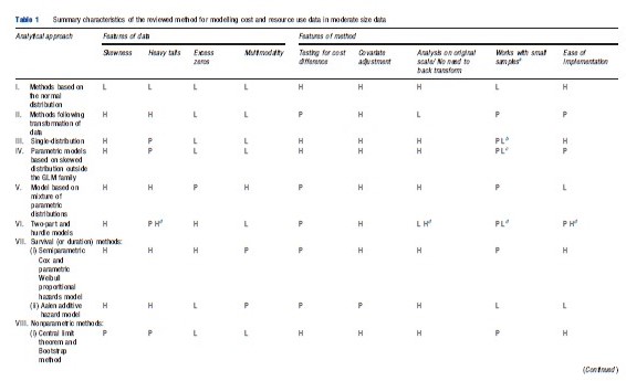
Their review identified 12 broad categories of methods: (I) methods based on the normal distribution, (II) models based on normality following a transformation of the data, (III) single-distribution generalized linear models (GLMs), (IV) parametric models based on skewed distributions outside the GLM family, (V) models based on mixtures of parametric distributions, (VI) two-part, hurdle and Tobit models, (VII) survival methods, (VIII) nonparametric methods, (IX) methods based on truncation or trimming of data, (X) data components models, (XI) methods based on averaging across a number of models, and (XII) Markov chain methods. Their recommendations were that, firstly, simple methods are preferred in large sample sizes (in the thousands) where the near-normality of sample means is assured. Secondly, in somewhat smaller sample sizes (in the hundreds), relatively simple methods, able to deal with one or two of the data characteristics studied, may be preferable but checking sensitivity of results to assumptions is necessary. More complex approaches for the analysis of mean costs in clinical trials that take into consideration the specific features of the data might lead to gains in precision and to more informative estimates if correctly specified, but run a risk of misspecification leading to biased results. Although some more complex methods hold promise for the future, these are relatively untried in practice and as such are not currently recommended for wider applied work.

One of the areas that Mihaylova et al. (2011) ruled outside of the scope of their review was the problem of censoring. However, particularly in the field of health economic evaluation conducted alongside clinical trials, the problem of censored cost data is highly prevalent. In the past, many analyses simply ignored this issue and presented analyses that assumed the data were uncensored. Fenn et al. (1995) argues that such an approach would lead to biased estimates of the true cost which, when adjusted for censoring, could be substantially higher. They went on to propose that standard survival analyses could be employed using the cost-scale in order to adjust for censoring. However, although this removed some of the problem, other authors demonstrated that the approach remained biased as the cost scale and the censoring event were no longer independent, an assumption required by the standard survival analysis methods.

Two general approaches have been shown to be capable of generating unbiased estimates of censored cost data. The first, known as the Kaplan–Meier Sample Average estimator is based on estimating a mean cost function over fixed time intervals based on the cost of the at risk population, then weighting those mean costs by the proportion surviving (estimated from the Kaplan–Meier survivor function) and summing across intervals to estimate total mean cost for the follow-up period. The other approach, based on Inverse Proportion Weighting (IPW) takes the inverse of the estimated survivor function for the censoring process as a weight to apply to the remaining observed data. Thus, at a given time point, if the censoring is 50% then each remaining data point receives a weight of 2 to reflect that the cost observed must count for both the observed subjects and the additional 50% that are censored at that point. The weighted costs in each time period are then summed and averaged to obtain the mean total cost.

These approaches can be extended into a regression framework in order to handle prognostic patient characteristics. Indeed, parameterizing the cost and survivor functions would also offer a crude approach to extrapolating beyond the data to estimate total lifetime cost. Although rarely acknowledged, the approach taken to estimating unbiased costestimates shares a common methodology with the estimation of quality adjusted survival analyses.

Other Forms Of Missingness

The problem of missing data is not new and has received much attention in the statistical literature as to the appropriate methods for handling missing data. Although in principle, missing economic data alongside clinical trials is no different to other forms of missing data; the distributional form of cost data (as presented above) may provide challenges for the analyst. Furthermore, because economic evaluation is commonly ‘piggy-backed’ onto clinical trials, there is a danger that economic variables will be considered less important by researchers responsible for data collection which could result in higher rates of missingness.

Missing data can arise in a number of ways. Univariate missingness occurs when a single variable in a data set is causing a problem through missing values, although the rest of the variables contain complete information. Unit nonresponse describes the situation where for some people (observations) no data are recorded for any of the variables. More common, however, is a situation of general or multivariate missingness where some, but not all of the variables will be missing for some of the subjects. Another common type of missingness is known as monotone missing data, which arises in panel or longitudinal studies, and is characterized by information being available up to a certain time point/wave but not beyond that point.

Little and Rubin (2002) outline three missing data mechanisms:

1. Missing completely at random (MCAR): If data are missing under this mechanism then it is as if random cells from the rectangular data set are not available such that the missing values bear no relation to the value of any of the variables.
2. Missing at random (MAR): Under this mechanism, missing values in the data set may depend on the value of other observed variables in the data set, but that conditional on those values the data are missing at random. The key is that the missing values do not depend on the values of unobserved variables.
3. Not missing at random (NMAR): It describes the case where missing values do depend on unobserved values.

The difference between these mechanisms is quite subtle, particularly for the first two cases of MCAR and MAR. Briggs and colleagues give the following example related to resource/ cost data. Consider a questionnaire distributed to patients, in order to ascertain their use of health care resources following a particular treatment intervention, where the response rate is less than 100%. The nonresponse is MCAR if the reason for failure to complete the questionnaire was unrelated to any prognostic variables in the data set. In practice, however, such a situation is unlikely. For example, retired patients may find more time to complete and return a questionnaire than those of working age. Also, being older on average, retired patients may make more use of health care resources. If having conditioned on the age and retirement status of the patients nonresponse is random then the missing data problem is considered MAR. However, it is possible that one of the reasons for nonresponse is that patients have been admitted to hospital. Now the missing data are NMAR because the value of the data that are not observed is driving the reason for nonresponse.

Note that the case of MCAR is quite rare – indeed the impact of administrative censoring is a special case of MCAR and survival analysis techniques employ the assumption that the censoring mechanism is independent of the event of interest when adjusting estimates for censoring. However, the case of NMAR is likely more common but difficult to demonstrate convincingly by the very nature of the problem of the values being related to the missing data problem. By far the majority of missing data methods relate to the attempt to correct statistically for the MAR case – using the observed data to predict the missing information in order to restore the full rectangular dataset for analysis. In general, multiple imputation, using a model-based imputation method is now readily implemented in most statistical packages and is a straightforward way to appropriately correct for the MAR problem. Alternatively, IPW approaches have been demonstrated to perform well and can obviate the need for creating multiple data sets to inform analyses.

Characterizing Uncertainty For Cost-Effectiveness Ratios

This section focuses specifically on uncertainty in the incremental CE ratio (ICER) statistic, defined as ICER = DC/DE, where DE is the per patient mean difference (treatment minus control) in effectiveness and DC is the mean per patient difference in cost.

Confidence Intervals/Surfaces For Incremental Cost-Effectiveness Ratios On The Cost-Effectiveness Plane

This subsection considers the presentation of uncertainty on the CE plane and the specific issue of calculating confidence intervals for CE ratios.

The Cost-Effectiveness Plane

The CE plane can be used to show the difference in effectiveness (∆E) per patient against the difference in cost (∆C) per patient. By plotting the effectiveness difference on the horizontal axis the slope of the line joining any point on the plane to the origin is equal to the ICER statistic.

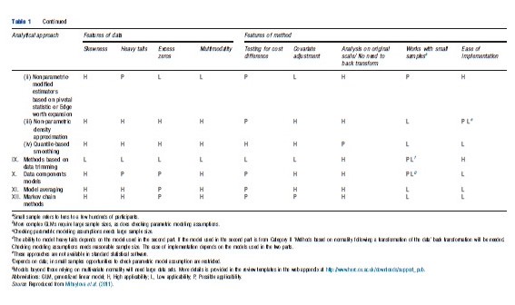
One treatment is said to ‘dominate’ another, being less costly and more effective, if it is located in the northwest (NW) quadrant or the southeast (SE) quadrant of the CE plane. In these two circumstances it is clearly appropriate to implement the dominant treatment and no estimation of CE ratios is required. However, far more common is for one treatment to be more effective but also more costly. In such circumstances, a decision must be made as to whether the additional health benefits of the more effective treatment are worth the additional cost. If the ICER of the more effective therapy (∆C/∆E) – the slope of a straight line from the origin that passes through the (∆E, ∆C) coordinate – is less than the acceptable ‘ceiling ratio’ of the decision maker (representing the willingness-to-pay for a unit of health gain) then the treatment should be adopted. This upper limit on CE can be given a value (R_c) and can be represented on the CE plane as a line passing through the origin with slope equal to R_c.

The use of the CE plane has previously been used to illustrate the CE of early endoscopy for dyspeptic patients versus no early endoscopy. In a clinical trial, the early endoscopy arm cost an additional ₤80 per patient and resulted in an additional 5% of patients free of dyspeptic symptoms at 12 months. This point is plotted on the CE plane in Figure 1 and the slope of the line joining that point to the origin represents the ICER of ₤1700 per patient free of dyspepsia at 12 months. Also shown on the CE plane are the standard confidence intervals for the difference in effect and difference in effect (the horizontal and vertical I bars respectively that cross at the point estimate). The box that is defined by these I bars (and which is also illustrated in Figure 1) represents an early attempt to approximate sampling uncertainty in the ICER. Nevertheless, subsequent methodological research has demonstrated the utility of two exact methods for confidence interval estimation – nonparametric bootstrapping or the parametric Fieller’s approach. These are described and illustrated for the dyspepsia trial below.

Fieller’s Theorem

Fieller’s approach is based on the assumption that the cost and effect differences follow a joint normal distribution, rather than the ratio itself.

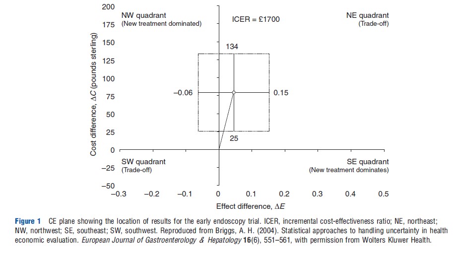
The standard CE ratio calculation of R=∆C/∆E can be expressed as R∆E – ∆C=0 with known variance R²var(∆E)+var(∆C) – 2R cov(∆E, ∆C). Therefore, a standard normally distributed variable can be generated by dividing the expression through by its standard error:

Setting this expression equal to the critical point from the standard normal distribution, z_a/2 for a (1-a)100% confidence interval, yields the following quadratic equation in R:

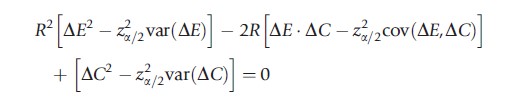
The roots of this equation give the Fieller confidence limits for the ICER.

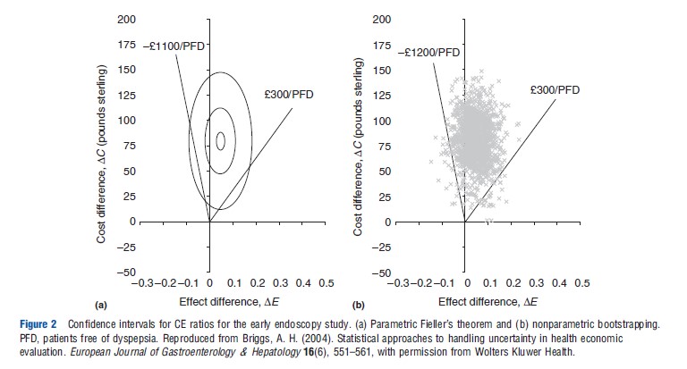
Figure 2(a) shows the assumption of joint normality on the CE plane for the early endoscopy example: three ellipses of equal density are plotted covering 5%, 50%, and 95% of the integrated joint density. Also plotted are the estimated confidence limits using Fieller’s theorem (d300 to d1100), represented by the slopes of the lines on the plane passing through the origin. Note that the ‘wedge’ defined by the confidence limits falls inside the 95% ellipse – this is because Fieller’s approach automatically adjusts to ensure that 95% of the integrated joint density falls within the wedge.

Bootstrapping

The approach of nonparametric bootstrapping is a re sampling procedure that employs raw computing power to estimate an empirical sampling distribution for the statistic of interest rather than relying on parametric assumptions. A number of authors have demonstrated its potential use for estimating confidence intervals for CE ratios. Bootstrap samples of the same size as the original data are drawn with replacement from the original sample and the statistic of interest is calculated. Repeating this process a large number of times generates a vector of bootstrap replicates of the statistic of interest, which is the empirical estimate of the statistic’s sampling distribution.

One thousand bootstrapped effect and cost differences for the early endoscopy example are plotted on the CE plane in Figure 2(b). Confidence limits can be obtained by selecting the 2.5th and 97.5th percentiles of the bootstrapped replications ordered from most favorable to least favorable CE ratio – this effectively ensures that 95% of the estimated joint density falls within the wedge on the CE plane defined by the confidence limits. As is clearly apparent from Figure 3(b), the bootstrap estimate of the joint density and the bootstrap confidence limits (₤300 to – ₤1200) are very similar to those generated by Fieller’s theorem.

Estimation Or Hypothesis Testing?

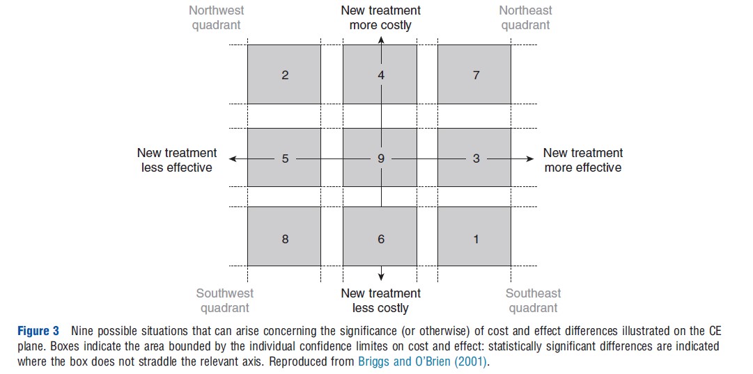
In practice, the example in Figure 1 is just one situation that can arise when analyzing the results of an economic analysis conducted alongside a clinical trial with respect to the significance or otherwise of the cost and effect differences. In fact, Briggs and O’Brien (2001) have argued that there are nine possible situations that could arise and these are illustrated on the CE plane in Figure 2 with multiple ‘confidence boxes’.

In situations 1 and 2, one intervention has been shown to be significantly more effective and significantly cheaper than the other and is therefore clearly the treatment of choice. In situations 7 and 8 one treatment has been shown to be significantly more costly, but also significantly more effective. It is in these situations that it is clearly appropriate to estimate an ICER and where much research effort has been employed to ascertain the most appropriate method for estimating the ICER confidence interval.

A potential problem arises in the situations where either the cost difference (situations 3 and 5) or the effect difference (situations 4 and 6) is not statistically significant. (The dyspepsia example falls into situation 4.) It is common to find analysts in these situations adapting the decision rule to focus only on the dimension where a difference has been shown. For example, it might be tempting in situation 4, as in the dyspepsia example, to assume early endoscopy has not better effectiveness than the no early endoscopy option and therefore focus the comparison only in terms of cost. This form of analysis – known as cost-minimization analysis – uses the logic that among outcome-equivalent options one should choose the less costly option.

The problem with this simple approach to decision making in situations where either cost or effect is not statistically significant is that it is based on simple and sequential tests of hypotheses. But the deficiencies of hypothesis testing (in contrast to estimation) are well known, and therefore the goal of economic evaluation should be the estimation of a parameter – incremental CE – with appropriate representation of uncertainty, rather than hypothesis testing.

Acceptability Curves

Although commentators are now largely agreed on the most appropriate methods for ICER confidence interval estimation, such intervals are not appropriate in all the nine situations outlined in Figure 3 above.

An important problem is that ratios of the same sign, but from different quadrants, are not strictly comparable. Negative ICERs in the NW quadrant of the plane (favoring the existing treatment) are qualitatively different from negative ICERs in the SE quadrant (favoring the new treatment) yet will be grouped together in any naıve rank-ordering exercise (note the treatment of negative ratios in the bootstrapping of the early endoscopy example above – because the negative ratios were in the NE quadrant they were ranked above the highest positive ratios to give a negative upper limit to the ratio). Similarly, positive ratios of the same magnitude in the SW and NE quadrants have precisely the opposite interpretation from the point of view of the intervention under evaluation. This is because the decision rule in the SW quadrant is the opposite of that in the NE. For example, an ICER of 500 may be considered as supporting a new treatment in the NE quadrant if society has set a ceiling ratio of 1000. However, in the SW quadrant this value of the ICER would be considered as support of the existing treatment rather than the new treatment. Again, any naıve ranking exercise could easily conflate ICERs with the same magnitude but with different implications for decision making.

Acceptability curves have been proposed as a solution to this problem. If the estimated ICER lies below some ceiling ratio, R_c, then it should be implemented. Therefore, in terms of the bootstrap replications on the CE plane in Figure 2(b), uncertainty could be summarized by considering how many of the bootstrap replications fall below and to the right of a line with slope equal to R_c lending support to the CE of the intervention. Alternatively, using an assumption of joint normality in the distribution of costs and effects, the proportion of the parametric joint density that falls on the cost-effective surface of the CE plane can be calculated. Because the appropriate value of R_c is itself unknown, it can be varied in order to show how the evidence in favor of CE of the intervention varies with the decision rule. The resulting acceptability curve for the early endoscopy example and based on the joint normal assumption shown in Figure 2(a) is presented in Figure 4.

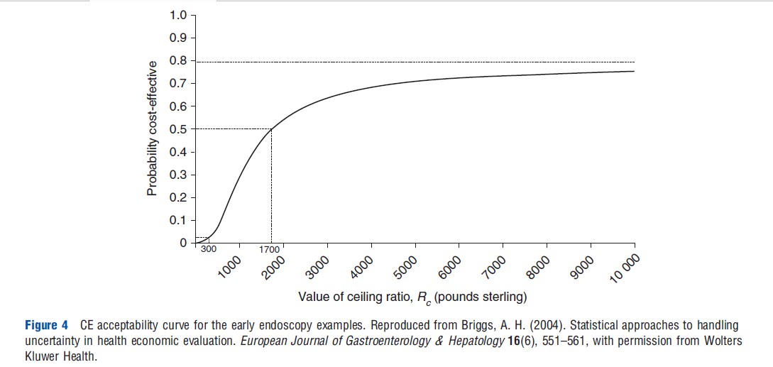
This ‘acceptability curve’ presents much more information on uncertainty than do confidence intervals. The curve cuts the horizontal axis at the p-value (one-sided) for the cost difference (which is p<.05 in the early endoscopy example) because a value of zero for R_c implies that only the cost is important in the CE calculation. The curve is tending toward one minus the p-value for the effect difference (which in the early endoscopy example is p=.20), because an infinite value for R_c implies that effect only is important in the CE calculation. The median value (p=.5) corresponds to the point estimate of the ICER, ₤1700 for the early endoscopy example.

As well as summarizing, for every value of R_c, the evidence in favor of the intervention being cost-effective, acceptability curves can also be employed to obtain a confidence interval on CE. The limits are obtained by looking across from the vertical axis to the curve at the appropriate points for the desired confidence level and reading off the associated CE value from the horizontal axis. For the early endoscopy example the 95% upper bound is not defined (because the curve is not defined at 0.975) and the 95% lower bound is equal to ₤300.

Development Of Net-Benefit Solutions

This section describes the reformulation of the standard CE decision rule into one of two possible net-benefit statistics. The use of the net-benefit statistic to estimate acceptability is highlighted, and the section goes on to describe regression approaches that utilize individual-level net-benefits to estimate CE directly.

Net-Benefit Statistics

The algebraic formulation of the decision rule for CE analysis that a new treatment should be implemented only if its ICER lies below the ceiling ratio, ∆C/∆E<R_c, can be rearranged in two equivalent ways to give two alternative inequalities on either the monetary scale (NMB) or on the health scale (net health benefit (NHB))

These decision rules are entirely equivalent to the standard rule in terms of the ICER but have the advantage that the variance for the net-benefit statistics is tractable and the sampling distribution of the net-benefits is much better behaved. The variance expressions for net benefits on the cost or effect scales are given by

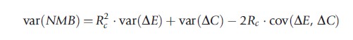
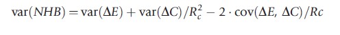
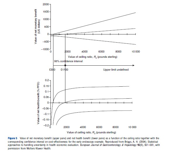
Because both the net-benefit statistics rely on the decision rule R_c to avoid the problems of ratio statistics, so the netbenefit can be plotted as a function of R_c. Both formulations of net-benefit are illustrated in Figure 5 for the early endoscopy example: the upper pane shows NMB and the lower pane NHB as a function of the ceiling ratio R_c. The net-benefit curves cross the horizontal axis at the point estimate of CE (₤1700 per patient free of dyspepsia). Where the confidence limits on net-benefits cross the horizontal axis gives the confidence interval for CE and this is shown between the two panes in Figure 5. The lower 95% confidence limit crosses the axis at ₤300, whereas the upper 95% limit does not cross the axis indicating that an upper 95% limit on CE is not defined for the early endoscopy example. Note the correspondence with the Fieller limits – this correspondence is explained by the fact that the two methods employ the exact same assumption of joint normality in costs and effects.

Acceptability Solutions

The net-benefit statistic provides a straightforward method to estimate the acceptability curve from Figure 4. The curve can be calculated from the p-value on the net-benefits being positive. Note that this gives the acceptability curve a frequentist interpretation, in line with the original paper that introduced the acceptability curve, although that same paper also labeled the vertical axis as ‘probability cost-effective.’ Strictly, such an interpretation requires a Bayesian view of probability, although it is straightforward to show that the frequentist curve based on the p-values for net-benefit and the Bayesian curve based on a normal likelihood and uninformative prior converge.

Regression Possibilities

The Section Net-Benefit Statistics illustrated how the ICER ratio statistic could be reformulated into a linear net-benefit statistic, by using the decision rule. Hoch and colleagues went on to demonstrate how the linearity of the net-benefit framework can be employed to directly estimate CE within a regression framework. By formulating a net-benefit value for each individual patient i as

where E_i and C_i are the observed effects and costs for each patient. At the simplest level, the following linear model

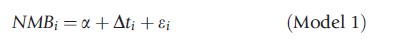
can be employed where a is an intercept term, t a treatment dummy taking the values zero for the standard treatment and one for the new treatment, and a random error term ε. The coefficient ∆ on the treatment dummy gives the estimated incremental net-benefit of treatment and will coincide with the usual estimate of incremental net-benefit obtained by aggregating across the treatment arms in a standard CE analysis. Similarly, the standard error of the coefficient is the same as that calculated from the standard approach. However, the power of the regression approach comes from the ability to covariate adjust (Model 2) and/or look at interactions between covariates and treatments to explore potential subgroup effects (Model 3).

These models are given algebraically below

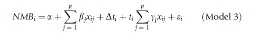
where there are p prognostic covariates x.

In the context of an experimental design like a randomized controlled trial, the randomization process is expected to ensure a balance of both observed and unobserved confounding factors across the treatment arms. In this case, the use of prognostic covariates will not materially affect the magnitude of the estimated CE, but may improve the precision of the estimate and lead to a corresponding narrowing of the estimated confidence intervals such that Model 2 should provide a more precise estimate of incremental net-benefit than Model 1.

The final term is the interaction between the treatment dummy and the prognostic covariates. The significance of the coefficients y_j on the interaction between the covariates of the model and the treatment dummy represent the appropriate test for subgroup effects – although this does not protect against spurious subgroup effects being detected by chance. Where treatment effect modification is detected, the fact that CE varies for different types of patient may have important consequences for decision making.

Despite the potential of using regression for net-benefit, the use of bivariate regression, through techniques such as seemingly unrelated regression, is more powerful, in that the same explanatory variables do not need to be specified for both cost and effect part of the equations.

Conclusions

This article has explored the development of statistical techniques for analyzing cost and CE data where individual data on coat and effect are available, often as a result of collecting patient-level data alongside a clinical trial. The statistical techniques for examining mean cost differences require subtle changes to the often standard approaches recommended in general (medical) statistics texts. This is due to the focus of CE analysis on informing decision making and maximizing potential health gain from available resources. Hence the focus on testing mean differences rather than reliance on rank order statistics, and the development of adaptations to the Kaplan–Meier approach to estimate cost in the presence of censoring. The net-benefit statistic is much better behaved than the ICER statistic when it comes to statistical analysis and representing uncertainty in CE estimates. Although most authors will want to continue to present results to their audience in terms of traditional ICERs, net-benefit statistics remain an important tool for the analyst to generate statistical measures of uncertainty.

Although this article has focused on the analysis of data on costs and effects generated alongside clinical trials, it is of note that CE analysis conducted within a decision modeling framework often employ individual patient data analyses to inform parameter estimates within the models. By using covariate adjusted parameter estimates, these decision models can explore the potential for patient heterogeneity in CE estimates. Statistical techniques can also be used at the patient level or study level for synthesizing multiple sources of evidence through traditional meta-analyses of network meta-analysis techniques.

The interested reader may also find the following articles of interest in terms of statistical methods for health economic evaluation:

• Economic evaluation alongside clinical trials: issues of design.
• Using observational studies in economic evaluation.
• Reviewing and synthesis of clinical evidence for economic evaluation.
• Analysis of uncertainty.
• Heterogeneity (including subgroup analysis).
• Value of information.

Bibliography:

1. Briggs, A. H. and O’Brien, B. J. (2001). The death of cost-minimization analysis? Journal of Health Economics 10(2), 179–184.
2. Fenn, P., McGuire, A., Phillips, V., Backhouse, M. and Jones, D. (1995). The analysis of censored treatment cost data in economic evaluation. Medical Care 33(8), 851–863.
3. Little, R. and Rubin, D. B. (2002). Statistical analysis with missing data, 2nd ed. Hoboken, New Jersey, USA: Wiley.
4. Mihaylova, B., Briggs, A., O’Hagan, A. and Thompson, S. G. (2011). Review of statistical methods for analysing healthcare resources and costs. Journal of Health Economics 20(8), 897–916.
5. Billingham, L. J., Abrams, K. R. and Jones, D. R. (1999). Methods for the analysis of quality-of-life and survival data in health technology assessment. Health Technology Assessment 3(10), 1–152.
6. Briggs, A., Clark, T., Wolstenholme, J. and Clarke, P. (2003). Missing presumed at random: Cost-analysis of incomplete data. Journal of Health Economics 12(5), 377–392.
7. Briggs, A. H., Wonderling, D. E. and Mooney, C. Z. (1997). Pulling cost-effectiveness analysis up by its bootstraps: A non-parametric approach to confidence interval estimation. Journal of Health Economics 6(4), 327–340.
8. Briggs, A. H. (2004). Statistical approaches to handling uncertainty in health economic evaluation. European Journal of Gastroenterology & Hepatology 16(6), 551–561.
9. Briggs, A. H. A. (1999). Bayesian approach to stochastic cost-effectiveness analysis. Journal of Health Economics 8(3), 257–261.
10. Chaudhary, M. A. and Stearns, S. C. (1996). Estimating confidence intervals for cost-effectiveness ratios: An example from a randomized trial. Statistics in Medicine 15(13), 1447–1458.
11. Delaney, B. C., Wilson, S., Roalfe, A., et al. (2000). Cost effectiveness of initial endoscopy for dyspepsia in patients over age 50 years: A randomised controlled trial in primary care. Lancet 356(9246), 1965–1969.
12. Etzioni, R. D., Feuer, E. J., Sullivan, S. D., et al. (1999). On the use of survival analysis techniques to estimate medical care costs. Journal of Health Economics 18(3), 365–380.
13. Hoch, J. S., Briggs, A. H. and Willan, A. R. (2002). Something old, something new, something borrowed, something blue: A framework for the marriage of health econometrics and cost-effectiveness analysis. Journal of Health Economics 11(5), 415–430.
14. van Hout, B. A., Al, M. J., Gordon, G. S. and Rutten, F. F. (1994). Costs, effects and C/E-ratios alongside a clinical trial. Journal of Health Economics 3(5), 309–319.
15. Kenward, M. G. and Carpenter, J. (2007). Multiple imputation: Current perspectives. Statistical Methods in Medical Research 16(3), 199–218.
16. O’Brien, B. J., Drummond, M. F., Labelle, R. J. and Willan, A. (1994). In search of power and significance: Issues in the design and analysis of stochastic cost-effectiveness studies in health care. Medical Care 32(2), 150–163.
17. O’Hagan, A. and Stevens, J. W. (2004). On estimators of medical costs with censored data. Journal of Health Economics 23(3), 615–625.
18. Stinnett, A. A. and Mullahy, J. (1998). Net health benefits: A new framework for the analysis of uncertainty in cost-effectiveness analysis. Medical Decision Making 18(supplement 2), S68–S80.
19. Tambour, M., Zethraeus, N. and Johannesson, M. (1998). A note on confidence intervals in cost-effectiveness analysis. International Journal of Technology Assessment in Health Care 14(3), 467–471.
20. Willan, A. R., Lin, D. Y., Cook, R. J. and Chen, E. B. (2002). Using inverseweighting in cost-effectiveness analysis with censored data. Statistical Methods in Medical Research 11(6), 539–551.