2. Perfectly Functioning Medical Labor Markets
Most governments regulate medical labor markets by licensing occupations, subsidizing medical education, encouraging labor to locate in underserved areas, and sometimes explicitly restricting entry. In order to understand the rationale for government regulation we begin by describing how a medical labor market with no market failures would function, using physicians as an example. We then describe the market failures that justify government regulation, and the implications of regulation on labor and, to a lesser extent, consumers.
2.1. Supply of Labor
The total number of hours of work physicians are willing to provide in a geographic market in a year depends on how many people chose to enter the profession in the past, how many decided to practice in a particular geographic market, and how many hours per year each physician decides to work. The following model of occupational choice is adapted from Rosen (1986). Assume, for simplicity, that there are only two occupations available to college graduates, medicine and law, and the same amount of graduate education is required for each occupation. People derive utility from consumption and the non-monetary attributes of a specialty, W. Examples of nonmonetary attributes include prestige, the intellectual content of an occupation, the types of consumers and colleagues one interacts with, and the flexibility of the work schedule. The expected lifetime difference in earnings between medicine (M) and law (L) is defined as ΔY5(YM 2 YL), and the equalizing difference is defined as Z. Z, which could be positive or negative, is the additional earnings an individual must receive in medicine in order to be exactly indifferent between entering the two occupations.
If the earnings difference between medicine and law (ΔY) exceeds a person’s given equalizing difference (Z), she will select medicine; otherwise she will select law. In equilibrium, all those selecting medicine will have a ΔY that exceeds their Z, and all those selecting law will have a ΔY that falls short of their Z. How many more students would choose to become physicians if the expected lifetime earnings in medicine increased due, for example, to an increase in the demand for physicians’ services? It will depend on how many students have an equalizing difference close to ΔY. The distribution of equalizing differences could have any shape; there is no reason, for example, to believe it will be normally distributed around ΔY. If there are a lot of students with a value of Z close to ΔY, then many more students will choose medicine over law when the expected earnings in the former occupation rise; the aggregate labor supply curve will be elastic. We review empirical estimates of the labor supply elasticity of physicians and nurses in section 3.
The model above is also relevant for examining whether a graduating medical student decides to enter a primary care versus a non-primary care specialty, how a new physician chooses a market in which to practice, and how a physician chooses a practice mode (e.g. solo practice versus group practice). In these cases Z represents the equalizing difference between practicing in one specialty versus another, the value of amenities in one area versus another, or the equalizing difference between practice modes. We review empirical estimates of the importance of expected earnings on physicians’ specialty choice and geographic location decisions in section 3.
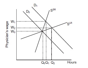
Short-run aggregate labor supply (SSR), depicted in Figure 1, will be steeper than long-run aggregate labor supply (SLR) due to the length of required medical training and costs associated with moving between geographic markets (or between specialties when examining the supply of specialty-specific hours). If the physician wage increases, more hours will be supplied in the short run as physicians who are already trained and practicing in a market decide to work longer hours. The long-run increase in hours will be greater as college graduates increasingly choose medicine over other professions and experienced physicians relocate to high-wage markets. The size and specialty mix of the physician workforce changes slowly over time because the flow of newly trained physicians from residency training is small relative to the stock of physicians (for example, 3 percent in the USA). In practice long-run supply may be dictated by the availability of medical school positions rather than student choices but we defer this discussion until section 3 because it is one implication of government regulation.
Figure 1
2.2. The Demand for Labor
In the Grossman (1972) model health has an investment and consumption value for consumers. Health cannot be purchased; it must be produced using medical care and a patient’s time as inputs. Medical care in turn consists of labor, medical devices, pharmaceutical products, and other technology. Consumers’ demand for medical care is thus derived from their demand for health (Grossman, 1972).
As Phelps (2010) points out, it is important to distinguish “…physicians as inputs into a productive process; physicians as entrepreneurs; and the final product of physician services, the actual event that involves patients.” A solo practicing physician is an entrepreneur who manages capital inputs, nursing and other labor inputs, and her own labor input. Physicians in group practices have the added challenge of designing incentives to manage many physicians’ inputs. We refer to the product provided by a solo physician or group practice as “physician services,” but clearly this consists of a combination of diagnostic tests, referral decisions, and procedures that may occur in the office, a separate outpatient facility, or a hospital. Physician services are produced with physician time, nurse time, other labor inputs, and capital. A group practice will hire physicians until the marginal revenue product equals the wage, w. The aggregate labor-demand curve depicted in Figure 1 (D0) is the summation of the firm-level marginal revenue products. Although we focus here on a group practice, the market wage represents the opportunity cost for a physician considering operating on her own in a solo practice or the amount offered by another group practice in the same city.
Consider a simple physician services production function with the only inputs being physicians and capital (K). Using the terminology in Hamermesh (1993), the price elasticity of labor demand, ηLL, is:
![]()
where s is the share of labor in total revenue (or costs), σ is the elasticity of substitution between labor and capital, and η is the product demand elasticity (i.e. the price elasticity for physician services in our example). Labor demand is relatively inelastic when labor’s share is high, it is difficult to substitute capital for labor, and demand for the final product is inelastic. The cross-elasticity of demand for labor in response to a change in the price of capital (or a different labor input in a more realistic production function), ηLK, is:
![]()
2.3. Equilibrium
Now consider a shift outward in the demand for physician services as a result of increased consumer income. Initially the quantity of services demanded will increase at the original prices; if supply is not perfectly elastic, as is assumed in Figure 1, prices will increase. A physician’s marginal revenue product increases as a result of the higher price of physician services in the output market, so the demand for physicians shifts from D0 to D1. Wages and the quantity of hours will rise in the short run to W1 and Q1, respectively. More college graduates will enter medicine now that ΔY has increased. If students have static or “cobweb” income expectations, they will expect the wage to remain permanently at W1. In this case supply will increase substantially in the long run, thereby creating a surplus of physicians, a subsequent reduction of the flow of students into medicine as the wage falls, and endless cycles of surpluses and shortages (e.g. Freeman, 1976). There is considerable empirical evidence, however, that the income expectations of prospective engineers, lawyers, and teachers are forward looking; they correctly anticipate that cohorts will arbitrage away temporary rents, and correctly expect the new long-run wage to be W2 (Ryoo and Rosen, 2004; Zarkin, 1985; Siow, 1984). In fact, Nicholson and Souleles (2001) find that medical students in the US anticipate future earnings changes when forming their own income expectations during the fourth year of medical school.
Labor surpluses and shortages will be self-correcting in efficient labor markets. If physicians are willing to supply more hours than firms are willing to hire at the prevailing wage, wages and physician incomes should fall. As the occupation becomes less attractive and fewer college graduates enter medicine, the reduced flow of newly trained physicians will increase wages and expected earnings until the financial return to medical education is once again commensurate with the return in other professions (adjusted by the equalizing differences). Conversely, if there is a shortage such that patients must wait months to schedule an appointment with a physician, consumers and/or health insurers will bid up physician fees, such that wages and physician earnings rise. Higher earnings will encourage a greater number of students to enter medicine until long-run supply again equals demand.