Spatial Econometrics

Spatial econometrics is concerned with measuring and modeling the correlation of observations generated by the inherent spatial structure of the data (Anselin, 1988). Such correlation, known as spatial dependence, may arise from local interaction of individuals, or from unobserved characteristics that are concentrated across space and that affect the variable of interest.

In health economics, spatial dependence may occur, for example, because individuals seek advice by speaking with neighbors regarding a variety of decisions concerning their health: the treatment to be purchased, the hospital wherein to be admitted, the diet to be undertaken. Local interaction can thus lead to an emergent collective behavior that empirically translates into a structure correlation among statistical units in the data. Spatial dependence may also arise if health providers engage in some forms of local strategic interactions, perhaps due to oligopolistic positions or agglomeration economies, when deciding the price to charge or the quality of health services to supply. At aggregate level of analysis, spatial correlation is likely to be present in the data if the investigator cannot observe important risk factors affecting the variable of interest, such as air pollution, migration, and criminality, which could be linked to regional rather than simply local trends, influencing prevalence and need across a wide geographical area. Spatial correlation can also be caused by a variety of measurement problems often found in applied work, or by the particular sampling scheme used to select units. An example is the lack of concordance between the delineation of observed spatial units, such as the region or the country, and the spatial scope of the phenomenon under study (Anselin, 1988). When the sampling scheme is clustered, potential correlation may also arise between respondents belonging to the same cluster. Indeed, units sharing observable characteristics, such as location or industry, may also have similar unobservable characteristics that would cause the regression disturbances to be correlated (Moulton, 1990).

This article provides a survey of econometric methods that are proposed to deal with spatial dependence in the context of linear panel data regression models. It then illustrates the application of spatial econometric methods to tackle problems in health economics. The discussion on these techniques is confined to linear panels with continuous dependent variable, whereas spatial discrete choice models will not be reviewed. Further, owing to space limitations, nonparametric methods for estimation of spatial models will not be discussed.

The plan of the remainder of the article is as follows. Section Spatial Weights and the Spatial Lag Operator introduces the notions of spatial weights and spatial lag. Sections Spatial Dependence in Panel Data Models, Estimation and Heterogenous Panels provide a review of spatial models and discuss their estimation under strictly exogenous regressors, whereas dynamic spatial models are treated in Section Dynamic Panels with Spatial Dependence. Section Testing for Spatial Independence introduces testing for spatial independence. Applications in health economics problems are reviewed in Section Applications of Spatial Econometrics in Health Economics, and Section Concluding Remarks concludes the article.

Spatial Weights And The Spatial Lag Operator

In spatial econometrics, the neighbor relation is typically expressed by the means of a nonnegative matrix, known as spatial weights matrix. In a spatial weights matrix, often indicated by W, the rows and columns correspond to the cross-section observations (e.g., individuals, regions, or countries), and the generic element, w_ij, can be interpreted as the strength of potential interaction between units i and j. The specification of W is generally arbitrary, typically based on some measures of distance between units, using, for example, contiguity or geographic proximity, or more general metrics, such as economic, political, or social distance. To avoid nonlinearity and endogeneity problems, spatial weights should be exogenous to the model, a condition that is not guaranteed when using more general distance metrics. By convention, the diagonal elements of the weighting matrix are set to 0, implying that an observation is not a neighbor to itself. Further, to facilitate the interpretation of estimates in spatial models, W is typically rowstandardized so that the sum of the weights for each row is 1, ensuring that all the weights are between 0 and 1. Finally, although most empirical works assume that weights are timeinvariant, these can vary over time.

An important role in spatial econometrics is played by the notion of spatial lag operator. Let zit be the observation on a variable for the ith cross-section unit at time t for i =1, 2,…, N; t =1, 2 ,…, T. Let z_t = (z_1t, z_2t,…, z_Nt)` , and W ¼={w_ij} be a time-invariant N × N spatial weights matrix. The spatial lag of z_t is given by Wz_t, with generic ith element

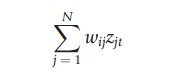
Hence, a spatial lag operator constructs a new variable, which is a weighted average of neighboring observations, with weights reflecting distance among units. The incorporation of these spatial lags into a regression specification is considered in the next section.

Spatial Dependence In Panel Data Models

Spatial Lag Models

Several problems in the social sciences require the inclusion in the regression model of spatial lags of the dependent variable among the regressors. Under this specification,

where x_it is a k×1 vector of observed regressors on the ith cross-section unit at time t, u_it is the error term, and p and β are unknown parameters to be estimated. The group effects, a_i, could be either considered fixed, unknown parameters to be estimated, or draws from a probability distribution. Section Estimation will discuss estimation under these two alternative frameworks. For the time being, it is assumed that regressors are strictly exogenous, and nonstochastic.

It is often convenient to rewrite eqn [1] in stacked form:

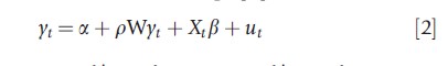
where y_t=(y_1t, y_2t,…, y_Nt)`, a = (a<sub>1</sub>, a<sub>2</sub>,…, a<sub>N</sub>)` , X_t = (x_1t, x_2t,…., x_Nt)`, and u<sub>t</sub> = (u<sub>1t</sub>, u<sub>2t</sub>,…, u<sub>Nt</sub>)` . Under certain asymptotic conditions on the spatial weights matrix, the correlation between the spatial lag of the dependent variable, W_yt and the error term, u_t, is nonzero, if p≠0. For this reason, conventional estimators of parameters p and β are inconsistent, and alternative estimation approaches, such as maximum likelihood (ML) and generalized method of moments (GMM), are needed.

Spatial Error Models

Another way to incorporate spatial dependence in the regression equation is by allowing disturbances to be spatially correlated. Consider the simple linear regression in stacked form:

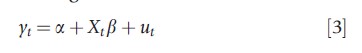
where the notation is as above. There exist few main approaches to assign a spatial structure to the error term u_t (as seen in Section Fixed effects specification, if a is assumed to be random, then a spatial structure could also be assigned to it); the intent is to represent the covariance as a simpler and lower dimensional matrix than the unconstrained.

One way is to define the covariance between two observations directly as a function of the distance between them. Accordingly, the covariance matrix for the cross-section at time t is E(u_tu`_y)=f (θ,W), where θ is a parameter vector and f is a suitable distance decay function, such as the negative exponential. The decaying function suggests that the disturbances should become uncorrelated when the distance separating the observations is sufficiently large. One shortcoming of this method is that it requires the specification of a functional form for the distance decay, which is subject to a degree of arbitrariness.

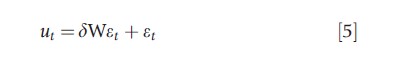
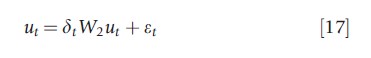
An alternative strategy consists of specifying a spatial process for the error term, which relates each unit to its neighbors through W. The most widely used is the Spatial Autoregressive (SAR) specification. Proposed by Cliff and Ord (1969), the SAR process is

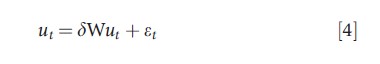
where δ is a scalar parameter, and ε_t = (ε_1t, ε_2t,…, ε_Nt)` , with ε_it~IID(0,σ²_εI_N). Other spatial processes suggested to model spatial error dependence, although less used in the empirical literature, are the Spatial Moving Average (SMA) and the Spatial Error Component (SEC) specifications. The first, pro-posed by Haining (1978), assumes that

where ε_t is as above. According to the SEC specification, introduced by Kelejian and Robinson (1995),

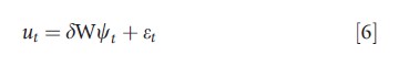
where ψ_t=(ψ_1t,ψ_2t,…,ψ_Nt)` and ψ_it~IID(0,σ²_ψ). A major distinction between the SAR and the other two specifications is that in the first there is an inverse involved in the covariance matrix. This has important consequences on the range of dependence implied by its covariance matrix. Indeed, even if W contains few nonzero values, the covariance structure induced by the SAR is not sparse, linking all the units in the system to each other, so that a perturbation in the error term of one unit will be ultimately transmitted to all other units. Conversely, for the SMA and SEC, the only off-diagonal nonzero elements of the covariance matrix are those corresponding to nonzero elements in W. Under certain invertibility conditions, spatial processes eqns [4]–[6] can all be written as special cases of the following general form

where R is a N×N matrix. For example, for an invertible SAR process R=(I_N-δW)^-1, whereas in the case of an SMA, R=I_N+δW.

Conventional panel estimators such as the fixed effects (FE) or random effects (RE) estimators of slope coefficients in eqn [3] with spatially dependent errors are √NT-consistent under broad regularity conditions and strictly exogenous regressors. However, these estimators are in general not efficient because the covariance matrix of errors is nondiagonal and the elements along its main diagonal are not constant.

Estimation of spatial models is considered next.

Estimation

Maximum Likelihood Estimator

The theoretical properties of quasi-ML estimator in a single cross-section framework have been studied by Anselin (1988) and Lee (2004), among others. More recently, considerable work has been undertaken to investigate the properties of ML estimators in panel data, in the presence of spatial dependence and unobserved time-invariant heterogeneity.

Fixed Effects Specification

For ML estimation of spatial regression models, it is convenient to consider the general case of a spatial lag model having SAR errors:

where the spatial lags in the dependent variable and in the error term are constructed using two (possibly different) spatial weights matrices, W₁ and W₂. Suppose that the group effects are treated as fixed and unknown parameters, and that ε_it ~IID(0,σ²_ε) Lee and Yu (2010a) propose a transformation of the above model to get rid of the FE, and then use ML to estimate the remaining parameters, p, β, δ, and σ²_ε. Specifically, the authors suggest to multiply all variables by a T×(T-1) matrix, P, having as columns, the (T -1) eigenvectors associated to the nonzero eigenvalues of the deviation from the mean transformation, M=I_T-1_T (1`<sub>T</sub> 1<sub>T</sub>)<sup>-1</sup>1`_T, where 1_T is a T-dimensional vector of 1. It is easily seen that 10 P= so that such transformation removes the individual-specific intercepts. After the transformation, the effective sample size reduces to N(T -1), and because P`P=I_{T -1}, the new error term has uncorrelated elements. Under some identification conditions, the estimator of the unknown parameters, obtained by maximizing the transformed model’s log-likelihood function, is consistent and asymptotically normal when either N or T, or both, are large.

Random Effects Specification

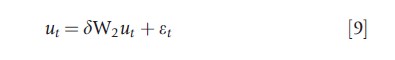
This formulation assumes that the group effects, a_i, are random and independent of the exogenous regressors. In this case, following Baltagi et al. (2009), a general specification can be suggested by assuming that spatial processes apply both to the random group effects and the remainder disturbances:

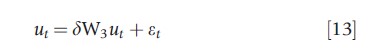
where μ=(μ₁, μ₂,…,μ_N)` , and it is assumed that μ_i~IID(0,σ²_μ) and ε_it~ IID(0,σ²_ε). The above model, by distinguishing be-tween time-invariant spatial error spillovers and spatial spillovers of transitory shocks, encompasses a variety of econometric specifications that are proposed in the literature as special cases. If the same spatial process applies to a and u_t (i.e., δ=y and W₂=W₃), this model reduces to that proposed by Kapoor et al. (2007); if y=0, it simplifies to that considered by Baltagi et al. (2003).

Consistency of estimator for the unknown parameters based on maximization of the model’s log-likelihood is established in Baltagi et al. (2009). A set of joint and conditional specification Lagrange Multiplier (LM) tests for spatial effects within the RE framework are proposed by Baltagi et al. (2009). These statistics allow testing model (10)–(13) against their restricted counterparts: the Anselin model, the Kapoor et al. models, and the RE model without spatial correlation.

Instrumental Variables And GMM

In the presence of heteroskedasticity, the ML estimator for spatial models under the incorrect assumption of spherical disturbances is generally inconsistent. As an alternative, instrumental variables (IV) and GMM techniques have been suggested.

In a single cross-section setting, Kelejian and Prucha (1998) propose a simple IV strategy to deal with the endogeneity of the spatially lagged dependent variable Wy_t that consists of using as instruments, the spatially lagged (exogenous) explanatory variable WX_t. The IV approach can be easily adapted in the context of spatial panel data models with either FE or RE. Hence, the Hausman’s specification test can be used to choose between FE and RE specification (Mutl and Pfaffermayr, 2011).

GMM estimation of spatial regression models for a single cross-section has been originally advanced by Kelejian and Prucha (1999). The authors focus on a regression equation with SAR disturbances and suggest the use of three moment conditions that exploit the properties of disturbances implied by a standard set of assumptions. Estimation consists of solving a nonlinear optimization problem, which yields a consistent estimator under a number of regularity conditions. Considerable work has been carried to extend this procedure in various directions. Liu et al. (2010) suggest a set of moments that encompass Kelejian and Prucha conditions as special cases. Kelejian and Prucha (2009) generalize their original work to include spatial lags in the dependent variable and allowing for heteroskedastic disturbances. This setting is extended by Kapoor et al. (2007) to estimate a spatial panel regression model with group error components and by Moscone and Tosetti (2011) for a panel with fixed effects. One advantage of the GMM procedure over ML is that it is computationally simpler, especially when dealing with unbalanced panels.

Heterogenous Panels

For panel data studies with large N and small T, observations are usually pooled and homogeneity of the slope coefficients is assumed. The latter is a testable assumption, which is often rejected in practice. A recent literature argues in favor of heterogenous estimates and suggests the following specification with heterogenous slopes

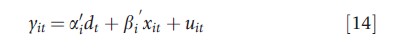
where d_t=(d_1t, d_2t ,…, d_nt)` is a n×1 vector of observed common effects (e.g., a time trend), x_it is a k-dimensional vector of strictly exogenous regressors, and β_i follow the random coefficient model β_i = β+v_i, with v_i~(0,Ω_v). It is further assumed that errors are generated by a spatial process having form (7), such as SAR, SMA, or SEC, where et follows a covariance-stationary process. Pesaran and Tosetti (2011) focus on estimation of the cross-section means of parameters, β=E(β_i), by conventional FE estimator, and by the following mean group estimator

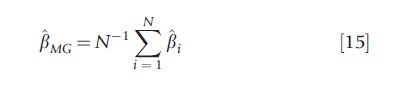
where

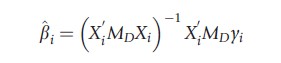
y_i= (y_i1, y_i2 ,…, y_iT)`, X<sub>t</sub>` =(x_i1, x_i2,…, x_iT ), MD =I_T -D(D`D)<sup>-1</sup> D`, and D`= (d₁, d₂ ,…, d_T). The authors show that under some regularity conditions, as N and T tend to infinity, β_MG , the asymptotic distribution of β_MG , (as well as that of the conventional FE estimator) does not depend on the particular spatial structure of the error, u_it, but only on Ω_v. Robust estimators for the variances of b^MG can be obtained following the nonparametric approach employed in Pesaran (2006). One advantage of this method is that it does not require a priori knowledge of the spatial arrangement of cross-sectional units. Indeed, misspecification of the spatial weights matrix may lead to substantial size distortions in tests based on the quasi-ML estimators of β_i (or β).

Temporal Heterogeneity

Temporal heterogeneity may be incorporated in a spatial version of the Seemingly Unrelated Regression Equations (SURE) approach, as suggested by Anselin (1988). This approach, suitable when N greatly exceeds T, permits slope parameters to vary over time, and errors are allowed to be both spatially and serially correlated. In its more general form, the spatial SURE is

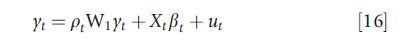
where β_t, p_t, and δ_t are time-varying parameters, and ε_t satisfies E(ε_tε`_s)=σ_tsI_N. Let Ω be a T×T positive definite matrix with elements σ_ts. ML or GMM techniques can be used to estimate the above model.

Dynamic Panels With Spatial Dependence

In the recent years, considerable work has been undertaken on estimation of panel data models that include both spatial and temporal dynamics. A variety of spatiotemporal models have been proposed in the literature. Consider the following general dynamic spatial panel:

The above model can be classified into different cases depending on the eigenvalue matrix of its reduced form. In particular, eqn [18] is stable if y+p+λ<1; spatial coin-tegration takes place when y+p+λ=1; whereas under the explosive case, y+p+λ>1. Under y+p+λ<1, Yu et al. (2008) derive the ML of the FE specification, showing that when T is large relative to N, the estimators are consistent and asymptotically normal, whereas when N/T>0, the limit distribution is not centered around 0, in which case, the authors propose a bias correction. Under y+p+λ=1, the ML estimator is consistent and asymptotically normal as in the stationary case, although spatial cointegration yields a singular asymptotic covariance matrix for the ML estimator. When y+p+λ>1, the ML is not tractable, although it turns tractable after applying a transformation that renders stable, the explosive variables (Lee and Yu, 2010b).

Testing For Spatial Independence

Spatial econometrics literature proposes a number of statistics for testing the null hypothesis of spatial independence, i.e., H₀: E(u_it u_jt) =0, i≠j in Model (3). The majority of these tests have been studied only in the case of a single cross-section. One of the most commonly used is the Moran’s statistic (Kelejian and Prucha, 2001), which, when extended to a panel set up, takes the form

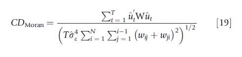
where σ²_ε is a consistent estimator for σ²_t, and u_t is a consistent estimator of regression errors. The CD_Moran is asymptotically normally distributed.

The information on the distance among units can also be used to build ‘local’ versions of some statistics as proposed in the panel literature to test against generic forms of cross-section dependence. For example, the local CD_P test proposed by Pesaran (2004) is

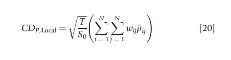
where S₀= ∑^N_i=1∑^N_j=1w_ij, and p_ij is the sample pairwise correlation coefficient computed between FE residuals of units i and j. The CD_P,Local test is asymptotically normally distributed. The reader is referred to Moscone and Tosetti (2009) for a review of this literature.

Applications Of Spatial Econometrics In Health Economics

The methods described in this article have been employed to study a variety of problems in regional and urban sciences, geography, economics, crime analysis, environmetrics, epidemiology, and public health. The recognition of a marked geographical concentration for many health indicators has encouraged a wide use of spatial methods to analyze health economics issues. This section first illustrates empirical evidence on spatial concentration for a number of health indicators, and then considers works on local interaction among healthcare providers.

Health Outcomes, Risk Factors, And Health Needs

There exists a growing literature adopting spatial econometric methods to model geographical clustering of various health conditions such as health status and mortality, obesity, and diseases, both communicable, like poliomyelitis, influenza, and HIV, and noncommunicable, like diabetes, cardiovascular problems, and mental health disorders. Lorant et al. (2001) study the impact on mortality of deprivation, measured by the Townsend index, and of a set of socioeconomic indicators, in Belgium at municipality level from 1985 to 1993. The authors estimate a spatial lag model and find evidence of high significant spatial effects (p=0.6) in mortality and of positive influence of deprivation on mortality. Chen et al. (2010) investigate the impact of access to chain grocers on body mass index (BMI) in Indiana (USA) in 2005. The authors estimate a spatial lag model by ML to control for possible ‘obesity epidemic’ effects, allowing the influence of access to chain grocers on BMI to differ depending on whether or not, a person lives in a low-income community. Empirical results suggest that improvement in access to chain grocer access significantly reduces the average BMI, in low-income communities. Congdon (2002) studies geographical variations in mental health outcomes proxied by hospital and community referrals for a set of diagnostic categories, using data on people living in a London health authority over the period 1994–99. Using Bayesian methods, the author derives an index of needs for mental health problems that includes spatial dependence and a set of sociodemographic variables, such as deprivation, community integration, and ethnicity. Hence, the author compares the forecasting performance of the developed index with that of traditional needs indices and shows that the forecast performance in predicting referrals improves consistently when accounting for spatial effects. One policy implication of the above studies is that formulae used to allocate healthcare resources across geographical areas could be ameliorated by incorporating spatial correlation.

Health Expenditure

Recent works in health economics and in the medical literature indicate that one important element explaining variations in health expenditure is represented by the spillover effect, that is, expenditure on health services in one locality can have beneficial or harmful effects across a wider geographical area. A number of factors can justify such wider effects. For example, a municipality may choose a particular course of action so as to persuade individual service users, families, or indeed service providing bodies, to migrate into or out of their area. Such flow can be encouraged by ensuring that health expenditure, clinical activity, or health policy is more (or less) attractive than that offered in neighboring authorities. Politicians may adopt this strategy as voters perhaps judge them relative to those in nearby localities. A municipality good (or bad) performance may encourage neighboring municipalities to mimic (or avoid) the activities and expenditure patterns associated with such performance.

A large number of papers have empirically tested the above hypotheses. One influential example is the work by Baicker (2005) that explores the extent to which health spending in one state is influenced by the spending in neighboring states. The author adopts IV and GMM approaches to estimate a spatial lag model for 48 contiguous US states, in the years from 1983 to 1992. One conclusion of this work is that states, in response to $1 increase in neighbors’ expenditure, raise their own expenditure by almost a full dollar. The reader is referred to Revelli (2006) and Moscone et al. (2007) for studies on the UK. Recent studies investigate the long-run dynamics of health spending. For example, Moscone and Tosetti (2010), using a panel of 49 US States over the period 1980–2004, estimate a regression equation for health spending assuming that errors are spatially correlated and also depend on a set of unobserved common factors. The authors find evidence of sizeable spatial correlation in health spending even after controlling for unobserved effects.

A number of works look at healthcare resources consumption and utilization rather than expenditure. For example, Filippini et al. (2010) study the demand of antibiotics in 240 Swiss regions in 2002. The authors estimate a spatial error model to account for infection spreading and find that dispensing practices induce higher rate of antibiotic consumption, even after controlling for patient characteristics, epidemiological variables, access to drug treatment, and spatial dependence. Joines et al. (2003) investigate the determinants of hospital admission rates in California and find significant spatial effects in hospitalization rates.

Hospital Competition And Agglomeration

Mobley (2003) adopts spatial econometric methods to study hospital competition under managed care in the State of California in the years 1993 and 1998. The author considers a SURE model with spatial lags of the dependent variable and estimates it by ML. Empirical results show that the price charged by a hospital is affected by the price set by neighboring hospitals, suggesting that such information may be used to design antitrust policies. Moscone et al. (2011) study hospital competition exploring the determinants of patients’ hospital choices, using 144

Italian hospitals in the years from 2004 to 2007. The authors conclude that the likelihood of choosing an hospital by an individual is significantly influenced by the experience in utilization of health services by patients living in the same postal code. However, the use of neighborhood information on average does not seem to lead patients to high quality hospitals. Cohen and Paul (2008) investigate why hospitals concentrate across territory, using data on 93 Washington state hospitals during 1997–2002. The authors estimate a system of cost function and input demand equations, which include an agglomeration variable as a cost shift factor, measured by the spatial lag of labor forces in neighboring hospitals. Results show significant agglomeration economies, perhaps due to cost saving generated by knowledge sharing with adjacent hospitals, labor market pooling, or lower employment search costs.

Concluding Remarks

This article has surveyed the most recent econometric methods for panel data dealing with spatial effects. Recent developments in spatial econometrics offer new methods for representing the spatiotemporal dynamics of many health economics phenomena. However, the range of spatial techniques adopted until now in health economics is rather limited, when compared to the methods developed in the literature. For instance, only few works have incorporated in their specification time-invariant unobserved heterogeneity and/or temporal dynamics. The use of recently developed techniques in spatial econometrics may offer insights and raise new questions in several areas of health economics.

Acknowledgment

The authors acknowledge the financial support from ESRC (Ref. no. RES-061-25-0317). They would like to thank the editor John Mullahy and Anirban Basu for their helpful comments on an earlier version of this article.

References:

1. Anselin, L. (1988). Spatial econometrics: Methods and models. Dordrecht, The Netherlands: Kluwer Academic Publishers.
2. Baicker, K. (2005). The spillover effects of state spending. Journal of Public Economics 89, 529–544.
3. Baltagi, B., Song, S. and Koh, W. (2003). Testing panel data regression models with spatial error correlation. Journal of Econometrics 111, 123–150.
4. Baltagi, B. H., Egger, P., and Pfaffermayr, M. (2009). A generalized spatial panel data model with random effects. CPR Working Papers No. 113. Syracuse, NY: Center for Policy Research, Maxwell School, Syracuse University.
5. Chen, S., Florax, R. J., Snyder, S. and Miller, C. C. (2010). Obesity and access to chain grocers. Economic Geography 86, 431–452.
6. Cliff, A. D. and Ord, J. K. (1969). The problem of spatial autocorrelation. In Scott, A. J. (ed.) London papers in regional science. London: Pion.
7. Cohen, J. P. and Paul, C. M. (2008). Agglomeration and cost economies for Washington. Regional Science and Urban Economics 38, 553–564.
8. Congdon, P. (2002). A model for mental health needs and resourcing in small geographic areas: A multivariate spatial perspective. Geographical Analysis 34, 168–186.
9. Filippini, M., Masiero, G. and Moschetti, K. (2010). Dispensing practices and antibiotic use. Working Papers no. 1006. Bergamo, Italy: Department of Economics and Technology Management, University of Bergamo.
10. Haining, R. P. (1978). The moving average model for spatial interaction. Transactions of the Institute of British Geographers 3, 202–225.
11. Joines, J. D., Hertz-Picciotto, I., Carey, T. S., Gesier, W. and Suchindran, C. (2003). A spatial analysis of county-level variation in hospitalization rates for low back problems in North Carolina. Social Science & Medicine 56, 2541–2553.
12. Kapoor, M., Kelejian, H. H. and Prucha, I. (2007). Panel data models with spatially correlated error components. Journal of Econometrics 140, 97–130.
13. Kelejian, H. H. and Prucha, I. R. (1998). A generalized spatial two stage least squares procedure for estimating a spatial autoregressive model with autoregressive disturbances. Journal of Real Estate Finance and Economics 17, 99–121.
14. Kelejian, H. H. and Prucha, I. R. (1999). A generalized moments estimator for the autoregressive parameter in a spatial model. International Economic Review 40, 509–533.
15. Kelejian, H. H. and Prucha, I. R. (2001). On the asymptotic distribution of the moran I-test with applications. Journal of Econometrics 104, 219–257.
16. Kelejian, H. H. and Prucha, I. R. (2009). Specification and estimation of spatial autoregressive models with autoregressive and heteroskedastic disturbances. Journal of Econometrics 157, 53–67.
17. Kelejian, H. H. and Robinson, D. P. (1995). Spatial correlation: A suggested alternative to the autoregressive model. In Anselin, L. and Florax, R. J. (eds.) New directions in spatial econometrics, pp. 75–95. Berlin: Springer-Verlag.
18. Lee, L. F. (2004). Asymptotic distributions of quasi-maximum likelihood estimators for spatial autoregressive models. Econometrica 72, 1899–1925.
19. Lee, L. F. and Yu, J. (2010a). Estimation of spatial autoregressive panel data models with fixed effects. Journal of Econometrics 154, 165–185.
20. Lee, L. F. and Yu, J. (2010b). Some recent developments in spatial panel data models. Regional Science and Urban Economics 40, 255–271.
21. Liu, X., Lee, L.-F. and Bollinger, C. (2010). Improved efficient quasi maximum likelihood estimator of spatial autoregressive models. Journal of Econometrics 159, 303–319.
22. Lorant, V., Thomas, I., Deliege, D. and Tonglet, R. (2001). Deprivation and mortality: The implications of spatial autocorrelation for health resources allocation. Social Science and Medicine 53, 1711–1719.
23. Mobley, L. R. (2003). Estimating hospital market pricing: An equlibrium approach using spatial econometrics. Regional Science and Urban Economics 33, 489–516.
24. Moscone, F., Knapp, M. and Tosetti, E. (2007). Mental health expenditure in England: A spatial panel approach. Journal of Health Economics 26, 842–864.
25. Moscone, F. and Tosetti, E. (2009). A review and comparison of tests of cross section independence in panels. Journal of Economic Surveys 23, 528–561.
26. Moscone, F. and Tosetti, E. (2010). Health expenditure and income in the US. Health Economics 19, 1385–1403.
27. Moscone, F. and Tosetti, E. (2011). GMM estimation of spatial panels with fixed effects and unknown heteroskedasticity. Regional Science and Urban Economics 41, 487–497.
28. Moscone, F., Tosetti, E. and Vittadini, G. (2011). Social interaction in patients’ hospital choice: Evidence from Italy. Journal of the Royal Statistical Society: Series A 175, 453–472.
29. Moulton, B. R. (1990). An illustration of a pitfall in estimating the effects of aggregate variables on micro units. Review of Economics and Statistics 72, 334–338.
30. Mutl, J. and Pfaffermayr, M. (2011). The Hausman test in a cliff and ord panel model. Econometrics Journal 14, 48–76.
31. Pesaran, M. H. (2004). General diagnostic tests for cross section dependence in panels. CESifo Working Paper Series 1229. Munich: CESifo Group Munich.
32. Pesaran, M. H. (2006). Estimation and inference in large heterogenous panels with multifactor error structure. Econometrica 74, 967–1012.
33. Pesaran, M. H. and Tosetti, E. (2011). Large panels with common factors and spatial correlation. Journal of Econometrics 161, 182–202.
34. Revelli, F. (2006). Performance rating and yardistick competition in social service provision. Journal of Public Economics 90, 459–475.
35. Yu, J., de Jong, R. and Lee, L. F. (2008). Quasi-maximum likelihood estimators for spatial dynamic panel data with fixed effects when both N and T are large. Journal of Econometrics 146, 118–137.