In problems studying the effects of a given intervention or treatment on health outcomes or health costs, it is often the case that researchers and analysts are faced with using observational study data to draw inferences. The use of such data gives rise to various concerns about biases that may influence treatment effect estimates. In the ideal world, one would be able to observe how an individual or agent would act under two scenarios – one where the agent had been treated and the other where the agent had not been treated. From here, estimating the effect of treatment on both the individual agent and population would be straightforward. Unfortunately, this is never a possibility in real-world settings.
To illustrate in more detail the difference between the ideal and real world, we can utilize the potential outcomes framework that has become popular in both statistics and econometrics in the past two decades. First, it is assumed that the study sample has N individuals. For each individual, we can define two potential outcomes, namely Yi(1) and Yi(0), which denote individual i’s outcome under the treatment and control conditions, respectively, for i=1,…,N. In the ideal world, we would be able to observe both Yi(1) and Yi(0) and we would directly know the effect of the treatment on individual i (namely, Yi(1) -Yi(0)). However, in the real world, it is usually observed that Yi=Yi (Zi), where Zi denotes whether the ith individual actually received treatment (Zi=1) or control (Zi =0) in practice. The value of Yi(1-Zi), commonly referring to as the counterfactual for the ith individual, is not observed. In most studies, researchers also observe (in addition to Yi and Zi) a set of pretreatment covariates or exogenous variables, Xi, which are assumed to be unaffected by treatment but that may predict the outcome Yi as well as whether the ith individual received the treatment or control condition. The variables in Xi are also commonly referred to as confounding factors or confounders because excluding them from an analysis examining the effect of Zi on Yi may lead to results from observational data in which the differences in the values of Xi between groups with Zi= 0 and Zi= 1 are combined with or confound the true causal effects of Zi on Yi.
With the potential outcomes framework in hand, we can now introduce a number of different types of treatment effects that a researcher may be interested in estimating in addition to the effect of the treatment on the ith individual (Yi(1)-Yi(0)). First, it is often the case that researchers are interested in estimating the population average treatment effect (PATE), which is defined as E[Y(1)- Y(0)], and tells us the impact of treatment on average over the entire population to which inferences are being drawn. Alternatively, it may be of interest to estimate the PATE for the treated (PATT), which is defined as E[Y(1)-Y(0)|Z=1], and tells us the average effect of treatment on individuals like those who actually receive treatment.
To estimate the PATE, the primary quantity of interest would be the sample average treatment effect (SATE), which equals 1/N∑Ni=1(Yi(1)-Yi(0)), and takes the average over the effect of treatment on all individuals in the sample. To estimate the PATT, the primary quantity of interest would be the SATE for the treated (SATT), which equals 1/NT∑τ:Zi=1(Yi(1)-Yi(0)), where NT denotes the number of individuals who are observed to receive treatment. SATT takes the average of the effect of treatment on all individuals in the sample who were observed to receive treatment. Both SATE and SATT are consistent (unbiased) estimates of PATE and PATT, respectively. However, it is never the case that one would be able to compute the SATE and SATT as only one of the two potential outcomes for each individual in the sample is usually observed.
A natural next step in trying to estimate PATE and/or PATT in practice would be to simply take the mean of Yi among those with Zi=1 and compare it to the mean of Yi among those with Zi=0. Unfortunately, this will only work if one has treatment and control conditions that are well balanced with regard to the distribution of all pretreatment factors that are known to be associated with the outcome. Such balance is hard to find when researchers are faced with using data from observational studies that do not randomize individuals in the sample to the treatment and control conditions. Moreover, usually only a handful of the pretreatment factors known to be associated with Y are actually available (i.e., those in X). Thus before estimating PATE and PATT, additional statistical and econometric methods must be utilized to achieve balance on the available pretreatment covariates or confounding factors, X, and additional assumptions must be made to ensure there is no residual confounding from imbalances in pretreatment covariates which were not observed. The rest of this article focuses on describing these assumptions and methods.
Critical Assumptions: Unconfoundedness And Overlap
Before introducing various methods that are available to researchers to achieve balance between individuals in the treatment and control conditions on the observed pretreatment covariates, X, when trying to estimate PATE or PATT, it is important to understand two key assumptions that are required to obtain consistent treatment effect estimates when faced with observational data.
The first key assumption goes by various names in the literature. It requires in layman’s terms that one has matched or balanced the individuals in the treatment and control conditions on values of X in such a way that there are no unobservable differences between the individuals in the two conditions after conditioning on X. In notational terms, we write this as (Y(1), Y(0))┴Z|X. The implication of this assumption is that systematic differences in outcomes between individuals with the same values of the pretreatment covariates are solely attributable to treatment. This assumption is commonly referred to as either the unconfoundedness assumption, selection of the observables, the conditional independence assumption, or ignorable treatment assignment. Throughout the remainder of this article, we will refer to it as the unconfoundedness assumption.
In principle, the unconfoundedness assumption is untestable. However, a number of approaches have been proposed that are useful for addressing its credibility, which revolve around the idea of doing sensitivity analyses to assess how sensitivity treatment effect estimates are to specific types of deviations from the unconfoundedness assumption.
The second key assumption required for consistent estimates of PATE or PATT using the methods discussed is the overlap assumption. The overlap assumption is formally written as 0<Pr(Z=1|X)<1. The implication is that one needs sufficient overlap in the distributions of the observed pretreatment covariates between individuals who are in the treatment and control conditions to be able to identify consistent estimates of PATE or PATT. Checking overlap is usually done by comparing the distribution of the estimated probability of receiving treatment conditional on X (commonly called the propensity score) among those in the treatment and control conditions to see if there is sufficient overlap in the estimated values of the measure; however, some promising work has been published which describes more formal ways to check overlap in the covariate distributions of the two conditions. Checking overlap is a critical step when estimating PATE and PATT. It is important to note that all is not necessarily lost if overlap is lacking. Assuming it is meaningful to do so, one may limit inferences to the average effect of treatment for the subset of the pretreatment covariate space where there is overlap.
Nonparametric Matching Methods
With our two key assumptions in hand, we now turn our attention to understanding ways in which researchers can try to balance the treatment and control conditions on the distributions of pretreatment covariates, X, so that consistent estimates PATE or PATT can be obtained. One of the most commonly used approaches for estimating PATE and PATT is to match individuals in the treatment and control conditions on values of X so that one can compare outcomes across pairs of matched treatment and control individuals with similar distributions of pretreatment covariates. Methods for creating meaningful matchings are numerous in the literature. This section focuses on the use of nonparametric matching techniques as nonparametric matching provides a method by which there are no restrictions on the functional form of the relationship between the outcome (Y), the treatment indicator (Z), and the pretreatment covariates (X). We begin by describing common techniques for one-to-one or pair matching (i.e., matching one control individual to one treatment individual) and then focus on the more elaborate techniques available for matching more than one individual to a given treatment or control individual.
The simplest case of one-to-one matching is exact matching which selects one control individual and one treatment individual so that they match exactly on X. Exact matching is only really feasible when the pretreatment covariates are all discrete (i.e., binary or categorical) and/or when one has only a handful of pretreatment covariates that need to be controlled for. In most other cases of one-to-one matching, the idea is to match one control individual with one treatment individual such that they have pretreatment covariates X whose values are within the same small neighborhood of each other. This type of matching (to no surprise) is commonly referred to as neighborhood matching or nearest neighbor matching.
The first step for any type of matching scheme (exact or neighborhood) is coming up with a meaningful distance metric that summarizes how close one individual is to another in terms of their values of X. There are generally three core types of distance metrics: categorical, caliper, and quadratic (including Mahalanobis distance). In each type, one begins by defining the distance between individual a in the treatment condition and individual b in the control condition using a specific formula. Here, the distance between individual a and individual b is denoted by δab. Categorical distance metrics are usually defined such that δab=1 if the covariates are an exact match and δab=∞ otherwise. Caliper distance metrics are defined such that δab=1 if |Xaj -Xbj|≤cj for all j where j=1,…,J and J denotes the total number of pretreatment covariates and dab ¼ N otherwise. Quadratic distance metrics are defined such that δab =(Xa-Xb)D(Xa -Xb)T and thus can take on any real number; Mahalanobis distance which defines D to the inverse of the variance–covariance matrix of X is an example of a quadratic distance.
Once the distance metric is defined, it is then computed for all possible pairs (a,b) of individuals, one in the treatment group and the other in the control condition and then an optimization algorithm selects the pairs that minimize the sum of dab across all pairs. From there, PATE and PATT follow directly by computing the treatment effect estimate for each pair and averaging across these estimates. The key difference in obtaining an estimate of PATE and PATT is in how the matching is done. For obtaining an estimate of PATT, one would aim to match each treatment case to a single control case and throw away all other controls which were not matched. For obtaining PATE, one would try to optimally match across both conditions without requiring that one condition is favored more than the other.
There is an extensive number of methods available for implementing one-to-one matching, including canned programs in most standard statistical software packages. However, there has also been extensive work done on matching algorithms which go beyond one-to-one matching, including matching one treatment individual with multiple controls (say two or three for each treatment individual) or matching each treatment individual to a variable number of controls in such a way that all control individuals are utilized. The ideas for these methods build off the theory described earlier in the article for one-to-one matching. However, it is important to note that matching methods that match a fixed number of controls to a single treatment individual tend to be criticized for being overly restrictive and for discarding data (namely, the unmatched control individuals). Various authors have shown that the use of a more flexible method, often called full matching, which makes use of all individuals in the data by forming a series of matched sets in which each set has either one treatment individual and multiple control individuals or one control individual and multiple treatment individuals is particularly effective at reducing bias due to confounding from pretreatment variables.
The section is ended by touching on the issue of how best to choose which pretreatment covariates that one should use in the matching algorithms described earlier in the article. It is generally recommended that variables chosen be predictive of both the outcome, Y, and the likelihood that the individual receives treatment, Pr(Z=1). Inclusion of irrelevant pretreatment covariates has the potential to impact both consistency and precision of treatment effect estimates.
Propensity Score-Based Methods
There is a second class of methods that are commonly used by researchers to handle the differences in the observed pretreatment covariate distributions among the treatment and control conditions. The class of methods differs from the methods presented in the previous section on Nonparametric Matching Methods because instead of matching on X directly, one matches on the predicted probability of receiving treatment, given the observed pretreatment covariates, commonly referred to as the propensity score. Matching on the propensity score as opposed to X greatly reduces the dimensionality problem of the nonparametric matching methods described earlier in the article. The theory shows that consistent estimation of PATE and PATT is possible when the treatment and control conditions are balanced with respect to the propensity score because balancing the two conditions on the propensity score in theory also balances the two conditions with respect to X.
Formally, the propensity score is denoted by e(x)=Pr(Z=1|X=x)= E[Z|X=x] and let e(x) denote the estimated propensity score (see below in this section for estimation). Various matching techniques (similar to those described earlier in the article) have become available for the case of trying to match treatment and control conditions on the propensity score in order to obtain consistent estimates of PATE and PATT. Each one is fundamentally based on the same ideas as the techniques for nonparametric matching on X, which are described earlier in the article except that things are much simpler when one only has to match on the single quantity of the propensity score rather than the entire vector of pretreatment covariates in X.
The most common approach for matching on the propensity score continues to be the nearest neighbor matching where a fixed number of controls, say k, are matched to one treatment individual and an optimal matching algorithm (as opposed to a greedy matching algorithm) are utilized to estimate PATT (as matching is driven by treatment individuals). The popular use of the nearest neighbor matching is likely a consequence of these algorithms being readily available in statistical software packages. However, as stated earlier in the article, such matching is suboptimal to full matching where a variable number of control individuals can be matched to a single treatment individual and a variable number of treatment individuals can be matched to a single control individual. The idea is that full matching forms the matched sets in an optimal way on the basis of the propensity score so that individuals from either condition who do not have many similar matches will not be forced to have bad matches as may happen when forcing all individuals to have a fixed number of controls. Unfortunately, software is not readily available to implement full matching in most software packages; the optmatch package available in R appears to be the only canned software currently available for implementing full matching.
The class of propensity score methods used to estimate PATE and PATT are not limited to matching. Commonly, both weighting by and subclassification on the propensity score are also used to obtain consistent estimates of PATE and PATT. With regard to weighting, one can consistently estimate PATE using the following formula:
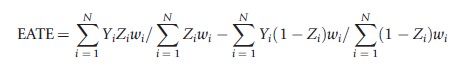
where wi=1/e(Xi) for those with Zi=1 and wi=1/(1-t(Xi)) for those with Zi =0. This estimate of PATE takes the difference in weighted means between those in the treatment and control conditions where the weights are set equal to the reciprocal of the estimated probability that an individual received the condition that they actually received. Such weights serve to make the distribution of observed pretreatment covariates, X, in each condition (treatment and control) look similar to the population’s distribution of X. The corresponding estimate of PATT is
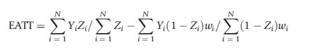
where wi=t(Xi)/(1-t(Xi)). This estimate for PATT takes the unweighted mean for the treatment condition and subtracts off the weighted mean for the control condition where the weights for the control condition equal the odds of an individual in the control condition being in the treatment condition. This weight serves to upweight control individuals who look more like individuals in the treatment condition and downweight those who do not in order to yield a consistent estimate of PATT.
With regard to sub-classification techniques based on the propensity score, the idea is to estimate the treatment effect of interest within subclasses that are defined based on the values of e(x) and to then aggregate across subclasses in a meaningful way to obtain final estimates of PATE or PATT. For example, it is generally the case that separate regression models on the outcome or mean differences between the two conditions are computed within each subclass and then results are aggregated across the subclasses by weighting those estimates by the subclass sample sizes if one is interested in PATE or the proportion of treatment cases in the subclass if one is interested in PATT.
A key issue for matching on, weighting by, or sub-classification on the propensity score, is how best to estimate the propensity score. In most applications, simple logistic regression (or parametric) models are utilized to estimate the propensity score. The treatment indicator, Z, is regressed on the pretreatment covariates X, possibly with or without interactions between the pretreatment variables and with limited attention paid to model selection procedures. In spite of the apparent ease of using logistic regression to estimate the propensity score, it is not the recommended method in the statistical and econometrics literature. Instead, use of more sophisticated semiparametric and nonparametric techniques are recommended. For example, it has been well established that machine learning methods outperform the use of simple logistic regression models in the binary treatment case. Machine learning methods work in an iterative fashion to fit nonparametric models to the predicted probability of receiving treatment. Use of conventional methods for estimating propensity scores such as logistic regression are less flexible than the machine learning techniques and typically require ad hoc variable selection procedures to reduce the number of degrees of freedom required by the pretreatment covariates and their interaction terms in the model. Such variable selection procedures risk biasing estimates of treatment effects because they can incorrectly omit covariates that are important to treatment selection. Similarly, variable selection procedures and the typical assumptions common in conventional modeling approaches risk model misspecification of the functional form of the relationship between the covariates and the treatment indicator, which can lead to very large biases in treatment effect estimate.
One example of a flexible, nonparametric machine learning technique that has been frequently utilized in the literature is the Generalized Boosted Model (GBM). GBM estimates the propensity score model using a flexible estimation method that adjusts for a large number of pretreatment covariates and which adaptively captures the functional form of the relationship between the pretreatment covariates and treatment selection with less bias than traditional approaches.
Use of propensity score weights has been shown to have a number of advantages over matching or sub-classification techniques based on the propensity score. In comparison to one-to-one or k-to-one matching techniques which throw away observations that do not match, weighting includes all observations in the outcomes analysis. In comparison with sub-classification techniques that require fitting multiple regression models to the outcome (one within each class), weighting techniques only fit one (weighted) regression model to the outcome which greatly minimizes variable selection issues and the need to tinker with the functional form. The main disadvantage of weighting is that it can be less efficient than matching or sub-classification, particular when good weights are difficult to obtain.
Doubly Robust Methods
We end this article by describing doubly robust methods that are commonly used to consistently estimate PATE and PATT. To put the goal of doubly robust methods in context, one must note that historically, the traditional approach for estimating PATE and PATT using observational study data was to utilize multivariable parametric regression models of the outcome (Y), which regress Y on the treatment condition
indicator (Z), and the observed pretreatment covariates (X), which were concerned to be potential confounders of the relationship between Y and Z. However, the assumptions of linearity (additivity) for the effects of the pretreatment covariates on Y was considered too rigid of an assumption and drew into question whether such models can yield consistent estimates of PATE and PATT giving raise to the nonparametric and propensity score methods described earlier in the article for obtaining consistent estimates of PATE and PATT. Although the methods described do not do any direct modeling of the outcome, they do come with their own assumptions, namely that the modeling done between the pretreatment covariates and treatment indicator are well specified. Doubly robust methods apply both techniques simultaneously (parametric regression modeling which control for X and matching or weighting the treatment and control conditions with respect to X) to produce consistent estimates of PATE or PATT as long as one of the two modeling approaches has been correctly specified. Thus, for example, use of both propensity score weighting and regression on the outcome with a parametric model leads to a doubly robust estimate of PATE or PATT because the estimates are consistent as long as one of the models is correct. Similarly, both matching on observed pretreatment covariates and controlling for those covariates in the outcome regression model fit to the matched pairs represent a doubly robust estimate of PATE and PATT assuming one of the two models is correct. Although doubly robust techniques can be less efficient if the parametric outcome model is correct, it is the final recommendation of this article that researchers go doubly robust whenever feasible to minimize the potential biases that could arise from using only a single technique.
References:
- Abadie, A. and Imbens, G. (2002). Simple and bias-corrected matching estimators for average treatment effects. NBER Technical Working Paper No. 283. Available at: http://www.nber.org/papers/t0283 (accessed 10.08.11).
- Hansen, B. B. and Olsen Klopfer, S. (2006). Optimal full matching and related designs via network flows. Journal of Computational and Graphical Statistics 15(3), 609–627.
- Heckman, J. J. (2008). Econometric causality. International Statistical Review 76(1), 1–27.
- Heckman, J. J., Ichimura, H. and Todd, R. (1998). Matching as an econometric evaluation estimator. Review of Economic Studies 65, 261–294.
- Hirano, K., Imbens, G. and Ridder, G. (2003). Efficient estimation of average treatment effects using the estimated propensity score. Econometrica 71(4), 1161–1189.
- Imbens, G. W. (2004). Nonparametric estimation of average treatment effects under exogeneity: A review. Review of Economics and Statistics 86(1), 4–29.
- Kang, J. D. Y. and Schafer, J. L. (2007). Demystifying double robustness: A comparison of alternative strategies for estimating a population mean from incomplete data. Statistical Science 22(4), 523–539.
- Lee, B. K., Lessler, J. and Stuart, E. A. (2010). Improving propensity score weighting using machine learning. Statistics in Medicine 29, 337–346.
- McCaffrey, D. F., Ridgeway, G. and Morrall, A. R. (2004). Propensity score estimation with boosted regression for evaluating causal effects in observational studies. Psychological Methods 9(4), 423–434.
- Ming, K. and Rosenbaum, P. R. (2001). A note on optimal matching with variable controls using the assignment algorithm. Journal of Computational and Graphical Statistics 10, 455–463.
- Rosenbaum, P. R. (1989). Optimal matching for observational studies. Journal of the American Statistical Association 84(408), 1024–1032.
- Rosenbaum, P. R. (1995). Observational studies. New York: Springer-Verlag.
- Rosenbaum, P. R. and Rubin, D. B. (1983). The central role of the propensity score in observational studies for causal effects. Biometrika 70, 41–55.
- Stuart, E. A. and Green, K. M. (2008). Using full matching to estimate causal effects in nonexperimental studies: Examining the relationship between adolescent marijuana use and adult outcomes. Developmental Psychology 44(2), 395–406.
- Zhao, Z. (2004). Using matching to estimate treatment effects data requirements, matching metrics, and Monte Carlo evidence. Review of Economics and Statistics 86(1), 91–107.