Models for Durations

Often one is interested in the time spent in a specific state and the effect of variables influencing the length of stay; for example, how long does a patient stay in a hospital and what is the effect of a medical intervention. The state can also be employment, and one may be interested in the effect of (changes in) health status on the probability that a worker leaves employment. Such processes are often described in the context of a duration model. In the duration models literature, the probability of leaving a specific state is referred to as the exit probability (in discrete time), or the exit rate or hazard rate (in continuous time). High exit rates are associated with short durations in the state and low exit rates with long durations.

Regression methods may not be useful in such applications. In practice, individuals are often observed for a limited time period, and, therefore, some individuals are not observed to have left the state of interest. Dealing with such censored observations is not straightforward in a regression model. It requires specifying a censored regression model, which often makes strong distributional assumptions. Furthermore, the value of some regressors may change over time. The health status of an individual can change during the course of an employment spell. It is unclear how one can include time-varying covariates in a regression model. Finally, a regression model considers only the mean duration. In applications one may be directly interested in the effect of a variable on the exit rate, or in the evolution of the exit rate over time. Example of the former is the effect of a drug on the recovery rate of a sick patient, or the effect of a health shock on the exit rate out of employment. These effects may be different early in the spell than later on.

This article reviews the literature with attention to empirical applications of such methods and the use of standard software such as STATA. The article will not fully cover all aspects of duration analysis. The remaining of this article is organized as follows. In the next section some formal concepts are introduced and simple nonparametric methods to describe duration data are provided. Section ‘Parametric and Semiparametric Models’ discusses different models used in applied duration analyses. Section ‘Unobserved Heterogeneity in Duration Models: The Mixed Proportional Hazard’ discusses the issue of unobserved heterogeneity in duration models. Section ‘Other Relevant Issues in Applied Duration Analysis’ provides a brief introduction to other relevant issues in the context of duration models, such as multiple spells, competing risks, and dynamic treatment evaluation.

Concepts And Nonparametric Estimates

Concepts

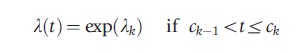
Let T be a nonnegative random variable representing the time spent in a specific state. This can, for example, be the length of an employment spell or the duration for which a person is sick. In practice, when there are individual data on durations, outcomes of this random variable are observed. The distribution function of this random variable is given by F(t)=Pr(T<t), which denotes the probability that the individual leaves the state within t time periods. The distribution function is uniquely characterized by the so-called hazard rate, which describes the exit rate out of the state at a point in time given that the individual is still in the state. The hazard rate is in continuous time the instantaneous exit rate at time t and is denoted by θ(t). In discrete time, θ(t)dt is the probability that an individual who did not leave before time period t leaves the state within a short time interval dt after time period t.

If the hazard rate is decreasing in t, then exiting the state becomes less likely the longer the individual is in the state. In case of sickness, one might expect to see such a decreasing pattern; individuals who have been sick for only a short period are more likely to recover than individuals who have been sick for a longer period. A decreasing pattern in the hazard rate is often referred to as persistence or state dependence. The complement of the distribution function 1-F(t) is referred to as the survivor function S(t). The survivor function describes the fraction of individuals who are still in the state after t time periods. This is thus the cumulative of not having left the state in all short time intervals before t. With high hazard rates, generally fewer people remain in the state when one proceeds over time; with low hazard rates, more people remain in the state. This illustrates the one-to-one relation between the hazard rate and the survivor function S(t) (and its complement F(t)).

Nonparametric Estimates Of The Hazard Rate: Bringing The Concepts To The Data

The appendix includes a link to a data set on individual sickness absence spells of teachers working in primary schools in the Netherlands. The data set includes individual sickness spells (t_i), an indicator whether or not the spell is right censored (d_i=1 for a completed spell and d_i=0 for a censored spell), and observed individual characteristics X_i. Censoring implies that recovery from sickness is not observed in the data. This may be the case because individuals are still sick at the end of the observation period, either because the observation window has ended or because the respondent leaves the sample (for instance, because she/he leaves the school). For now it is assumed that the censoring mechanism is independent of the outcome variable of interest (the issue of independent censoring will be elaborated in Section ‘Other Relevant Issues in Applied Duration Analysis,’ where competing risks models is discussed). To define in STATA that one is using duration data, the command stset spell-length, failure(failed) should be used. Some elements of X_i may change over time, but for now it is assumed that these are fixed as of the start of the spell. The sickness spells in the data are all observed to start during the observation window. In the literature this kind of sampling scheme is referred to as a flow sample.

With data as described above, one can obtain a nonparametric estimate of the hazard rate. Recall that the intuition of the hazard rate is that it describes exit probabilities in short time intervals, given that the individual has not left the state before the start of the interval. Therefore, as a simple and direct estimate of the hazard rate after t time periods, one can take the ratio of the number of observed exits in the next short time period as a fraction of the number of individuals who are still in the sample at the start of the interval. Or in more technical terms,

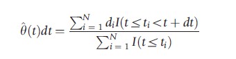
The denominator is referred to as the risk set, i.e., those individuals who are still in the state at time period t and who are ‘at risk’ of leaving the state.

Often not only the hazard rate is of interest, but also the survivor function is estimated. Given the one-to-one relation between the hazard rate and the survivor function, the latter can be estimated using the estimated hazard rates. If it is imposed that the unit of time dt is 1, then the fraction surviving after the first period S(1) is the fraction of people who have not left the state in the first period: 1 –θ(1). The fraction surviving after two periods S(2) equals (1-θ(1)*(1-θ(2)), and so on. There are alternative formulations for the nonparametric estimation of the survivor function. Most statistical software packages report the popular Kaplan–Meier estimator.

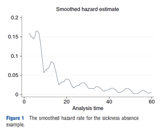
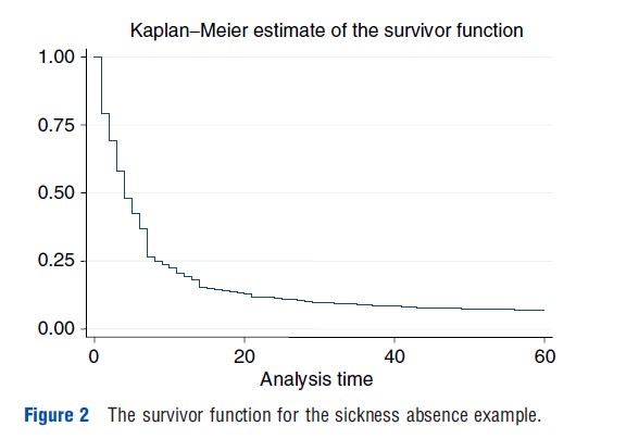
In STATA sts list should be used to get estimates of the hazard rate and the survivor function. With sts graph the Kaplan–Meier estimate for the survivor function is plotted. And sts graph, hazard plots the smoothed empirical hazard rate. Figure 1 shows the smoothed hazard rate for the data on sickness absence of teachers for the first 60 days. The figure shows a high recovery rate quickly after the start of sickness absence and declining hazard rates with occasional jumps thereafter. The declining hazard rate suggests state dependence. It may be that for each individual, recovery becomes more unlikely as time proceeds. Alternatively, there could be dynamic selection: those with less serious illnesses leave the state first, so that in the end the most serious cases remain. This illustrates that the nonparametric methods are useful for summarizing the data, but that it is important to control for heterogeneity within a sample of individuals. This is discussed further in the next section. Figure 2 shows the Kaplan–Meier estimate of the survivor function. At the start all individuals are present (at t =0, S(t)=1), and as time proceeds, more and more people leave the state. Note that, as expected, the high hazard rates in the beginning lead to a steep decline in the survivor function and the lower hazard rates later in time lead to slower decline in the survivor function.

Often, data describe different groups. For example, the data may contain sickness durations of individuals who received some treatment and of individuals who did not receive this treatment, or sickness absenteeism spells of teachers in different schools. One might be interested in whether or not hazard rates differ between groups. This can formally be tested using Logrank tests, which are nonparametric tests for the null hypothesis that the survival functions describing the durations in the different groups are identical. The underlying idea of the Logrank tests is that the order in which individuals exit the state is random in case the different groups have the same survival function. If after t time periods an exit is observed in one of the two samples, under the null hypothesis, the probability that the exit occurred in the first sample is simply the number of survivors in the first sample after t time periods as a fraction of the total number of survivors in both samples at this moment. The Logrank test is based on evaluating these probabilities for all observed exits in the data. It can also be used in case the data contain more than two groups. In STATA the comment sts test strata is used to perform Logrank tests, where the variable strata denotes the different groups. Finally, if the data do not contain any censored observations, the ranksum test can also be used.

Parametric And Semiparametric Models

Parametric Models

The previous section mentioned that state dependence implies that the hazard rate is decreasing in the time spent in the state. There can be two reasons for observing state dependence. First, individual hazard rates are decreasing over time, which implies that for each individual, exit becomes less likely the longer the individual has already been in the state. So in case of sickness this implies that for each individual it is the case that she/he is more likely to recover in the next period if the sickness spell is still short than when the sickness spell is further progressed. The second reason for observing state dependence is dynamic selection, which means that individuals with good characteristics (i.e., with high exit rates) leave the state early. So the longer is the duration, the more the sample of survivors will move toward individuals with bad characteristics and consequently low exit rates. Also dynamic selection implies that (overall) hazard rates decrease in the elapsed duration.

In many settings, both causes for state dependence have different implications for public policy. To analyze how important both mechanisms are, often more structure is imposed on the hazard rates. A popular specification is the so-called proportional hazard (PH) specification:

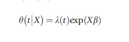
The function λ(t) is the baseline hazard. This describes duration dependence common to all individuals, which does not vary with individual characteristics. So a declining baseline hazard is the first explanation for observing state dependence. The role for regressors X is in the regression function exp(Xβ), which is specified such that it is nonnegative. The latter is required because hazard rates cannot be negative. The PH assumption implies that the ratio of the hazard rates of two individuals is constant over time. At any moment in time, individuals with good characteristics are more likely to leave. So when the elapsed duration is progressing, the composition of survivors moves more toward individuals with bad characteristics. The presence of heterogeneity, therefore, always causes aggregated hazard rates to decline.

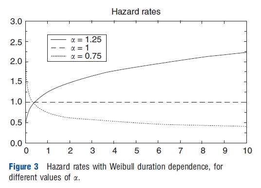
The most straightforward way to estimate duration models is by using maximum likelihood. However, in the case of the PH model, this also requires parameterizing the baseline hazard. A simple parametric function is provided by the Weibull distribution, λ(t)=at^a-1. This specification imposes a monotonic relationship for the effect of time on the hazard rate. For a>1 the hazard rate increases with time (positive duration dependence), for a<1 the hazard rate decreases over time (negative duration dependence), and for a=1 the hazard rate is constant over time (exponential distribution). This is illustrated in Figure 3.

In STATA, PH models can be estimated using the command streg varlist, distribution (Weibull) nohr. Varlist is the set of observed characteristics included in X. The baseline hazard follows a Weibull distribution, but also other specifications can be used. For example, a log-normal specification allows for a nonmonotonic pattern of duration dependence. Finally, nohr ensures that in the output, the parameter estimates for β are reported rather than hazard ratios.

Semiparametric Models: Piecewise Constant Specification Of The Baseline Hazard

Maximum likelihood estimation provides only consistent estimators if the model is specified correctly. Most choices for the baseline hazard involve specific functional forms and these may be too restrictive. For example, the Weibull distribution assumes that the hazard rate is constant, monotonically increasing or monotonically decreasing. This assumed duration dependence pattern may be violated in practice and will then lead to inconsistent estimates of the regression parameters b. Heckman and Singer (1984) provide a piecewise constant specification for the baseline hazard, which minimizes the distributional assumptions. The idea is that the baseline hazard takes different values on prespecified time intervals:

For k =1,2,…,K, with c₀, the lower bound, set to zero and c_K, the upper bound, set to infinity. The λ_ks are parameters to be estimated along with the regression parameters β. The cutpoints c_k are chosen in advance by the researcher. The piecewise constant specification requires a normalization. Either one can exclude an intercept from the regression function exp(Xiβ), or a restriction should be imposed on the λ_ks. Most straightforward is to fix λ₁ =0.

The key advantage of the piecewise constant specification is that by making the intervals very small, the specification can approximate any function arbitrarily close. In practice, when estimating a PH rate model with piecewise constant duration dependence, in each interval at least some exits should be observed. If there are no exits in an interval, the parameter λ_k cannot be estimated. Furthermore, without making strong extrapolation assumptions, the duration dependence pattern cannot be estimated beyond the latest observed exit in the data. This implies that after estimating the model, it is, for example, difficult to estimate the expected duration. Consequently, it may be preferable to present estimates of the median or other quantiles of the distribution. In practice when estimating hazard rate models with piecewise constant duration dependence, it is advised to start with a very small number of broad intervals, and subsequently split intervals until no substantial improvement in the model is found. A complication is that most statistical software packages, such as STATA, do not directly allow for the option of piecewise constant duration dependence. However, in case one divides the data in discrete time intervals (such as weeks or months), the piecewise constant duration dependence translates into different intercepts for each time interval. STATA can handle time-varying regressors. The next section elaborates on the issue of time-varying regressors.

Semiparametric Models: Cox’s Partial Likelihood

Even though one can try to minimize the distributional assumptions by choosing, for example, piecewise constant duration dependence, the maximum likelihood estimation requires the full specification of the hazard rates. The risk of misspecification, therefore, always remains present. An alternative estimator can be based on the rank order in which individuals exit the state. If t₍₁₎ describes the shortest observed duration in the sample, then the probability that individual i leaves the state at t₍₁₎ conditional that someone leaves at t₍₁₎ equals

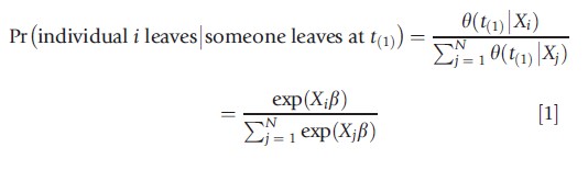
This probability is thus the ratio of hazard rates of individual i and the sum of all individuals in the risk set. Owing to the proportionality of the hazard rate, this probability does not depend on the baseline hazard λ(t). This holds not only for the shortest duration in the spell. For all observed completed durations, the probability that a specific individual exits is the ratio of the regression function for this individual over the sum of regression functions of all survivors at that duration. Cox partial likelihood estimation only evaluates points where exits are observed in the data, and uses the probabilities provided in eqn [1] above. So without making any functional form assumptions on the baseline hazard, the parameters β can be estimated. In STATA the command stcox varlist, nohr is used for partial likelihood estimation.

Because partial likelihood estimates only β, the estimation results cannot be used for making predictions on durations, such as computing median durations (for individuals with specific characteristics). If one wants to make such predictions or is interested in the duration dependence pattern, the baseline hazard should be estimated. The Breslow method gives a procedure to retrieve the baseline hazards after partial likelihood estimation. To obtain the estimate for the baseline hazard in case of partial likelihood estimation in STATA, the options basehc (hazard) and basesurv (survivor) can be used.

Additional Complications In Estimating Duration Models

So far this article made the implicit assumptions that each spell is followed from the inflow in the state, that one observes the exact duration of the spell, that censoring is exogenous, and that individual characteristics remain constant during the spell. Next, the article briefly discusses the consequences if the data do not fit these assumptions.

Duration data may not be registered in continuous time, but describe in which time interval a spell ends. For example, the NFHS India describes for child mortality, the exact day of death if a child died within the first months after birth, the months of death if the child died between 1 month and the first birthday, and the year of death if the child died after the first birthday. In such cases the appropriate likelihood contribution should be based on the probability statements associated with such observations. Unfortunately, statistical software packages such as STATA do not handle this in their standard commands.

More problematic is the case in which spells are not followed from the inflow in the state. When, for example, looking at mortality rates of older individuals, often the data describe individuals who were at some calendar time older than a particular age. Or when looking at transitions out of employment into retirement, the data may contain a sample of older persons who are still working. These kinds of samples are referred to as stock samples, because they describe at a specific calendar time the stock of individuals who are in a state. Inference using stock samples is more complicated than using inflow samples. In stock samples individuals with bad characteristics (for leaving the state) are overrepresented. Individuals with bad characteristics experience, on average, longer time periods in the state. Therefore, they are more likely to be in the state at the calendar time of sampling and thus to be included in the stock sample. For example, when considering individuals on sickness absenteeism at a specific calendar time, this will include a relatively large share of long-term sick people, so people with more serious conditions.

In the most general set-up, a stock sample includes retrospective information (the elapsed duration e that an individual already has been in the state) and prospective information (residual duration r beyond the time of sampling). Inference can be based on the retrospective information, the prospective information, or both retrospective and prospective information. The expressions for the likelihood function become cumbersome and cannot be estimated with standard software in all but one case: the case in which one looks at the distribution of the duration r conditional on the elapsed duration e. This can be implemented in STATA by using the subcommand origin of the stset command.

So far it was assumed that censoring (d_i=0) is independent of the duration of interest (T). This may not always be the case. For instance in a clinical trial, terminally ill patients may be removed from the trial before the trial has ended. In this case the censoring is informative on the hazard rate. In case censoring is not exogenous, competing risks models should be used. Section ‘Other Relevant Issues in Applied Duration Analysis’ briefly discusses this.

Finally, until now it was implicitly assumed that the vector X includes only variables that are constant from the start of the spell, but some characteristics may change over time. For instance, time spent in employment may depend on the health and the health status may change over time, or individuals may move to another region. The hazard rate can easily be modified to allow for time-varying characteristics. For example, one can write the PH rate as θ(t|X_i(t))=λ(t) exp(X_i(t)β) and the discussion above still applies. However, exogeneity of the regressors becomes an issue. The process X(t) must be (weakly) exogenous, implying that values of X(t) are only influenced by events that have occurred up to t and these events are actually observed. In the example of healthy lifetime, this excludes the situation where the individual knows that future health will fall (e.g., because of a chronic illness) and in anticipation reduces hours worked (X(t)). The article returns to this in Section ‘Other Relevant Issues in Applied Duration Analysis’ when discussing dynamic treatment evaluation. In case the exogeneity condition holds, STATA can be used for estimating. See the stsplit command in STATA to reorganize the duration data so that one can deal with time-varying covariates.

Unobserved Heterogeneity In Duration Models: The Mixed Proportional Hazard

Often the vector of observed characteristics X does not contain all variables relevant for leaving the state. For instance, in the context of individual lifetime, genetic factors may be relevant but unobserved, and the same may hold for factors like time preference or risk attitude driving health investment behavior. Ignoring unobserved heterogeneity causes the models to fail to control for dynamic selection, and thus the estimator for the baseline hazard λ(t) will be inconsistent. Incorrectly ignoring the presence of unobserved heterogeneity not only generates spurious duration dependence, but also the estimates of β are biased toward zero. The latter holds even if the unobserved heterogeneity is orthogonal to the variables included in X. Therefore, one would like to allow for the presence of unobserved heterogeneity within the hazard rate.

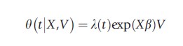
Let V describe the unobserved characteristics in the hazard rate, and it is assumed that unobserved characteristics V are independent of observed characteristics X, i.e., V┴X. The unobserved factors are random effects and follow at inflow (t=0) in the state a distribution G(v). The individual exit rate is often specified using a mixed proportional hazard (MPH) specification:

As time proceeds, individuals with good characteristics (high values of V) are more likely to leave the sample. This implies that among the survivors at time t, individuals with bad unobserved characteristics will be overrepresented. And the longer the time period t, the more the sample of survivors will move toward individuals with bad characteristics. This will lead to a discrepancy between the inflow distribution G(V) of V and the distribution of V among the survivors in the sample (G(V|X, T≥t)). As time proceeds, the observed hazard θ(t|X) declines faster than the baseline hazard λ(t).

In the presence of unobserved heterogeneity, the observed hazard rate y(t|X) does not factorize into t and X anymore. Therefore, it is not possible to use Cox’s approach to eliminate the baseline hazard from the partial likelihood function. This implies that maximum likelihood estimation should be used. In STATA the command streg varlist, duration (Weibull) fraily(gamma) nohr can be used to optimize this loglikelihood function. It is, however, necessary to specify the unobserved heterogeneity distribution G(v), for example, a gamma distribution. Furthermore, two normalizations are necessary on the duration dependence l(t), the regression part exp(X_iβ) and the mean of the unobserved heterogeneity E[V] in the inflow.

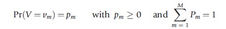
Misspecification of G(V) leads to biases in the estimators for λ(t) and β if there is substantial censoring in the data. Furthermore, misspecification of λ(t) usually causes significant biases in the regression parameters. It is therefore advisable to use flexible functional forms for the mixing distribution and for the baseline hazard. The previous section already introduced the piecewise constant specification as very flexible for the baseline hazard. Usually a mass-point distribution is considered to be the most flexible distribution for the unobserved heterogeneity. The idea is that V can take M different values, each acting as constants on the hazard rate:

In theory any distribution can be approximately arbitrarily close if M is chosen to be sufficiently large. However, in most applications M does not exceed 3. STATA does not have a command for a mixing distribution with discrete mass points. When optimizing the loglikelihood function, it is advised to start with a small M and then to add new points until the loglikelihood function does not improve anymore. The latter often implies either that new points have a very small probability mass or that the location of two mass points converge toward each other.

Other Relevant Issues In Applied Duration Analysis

Multiple Spells

So far it was implicitly assumed that for each individual only one spell is observed. However, it may be that the data contain multiple spells sharing the same unobserved component. For example, because within the observation period many workers experience multiple spells of sickness absenteeism, or because children born in the same family have the same unobserved component when modeling child mortality.

To formalize multiple spells, consider a cluster c=1,…,C containing I_c observed spells. The hazard rate of observation i=1,…,Ic in cluster c equals

Each cluster is allowed to have a separate baseline hazard λ_c(t) including duration dependence, cluster fixed effects, and possible interactions between both. To estimate the regression parameters β, stratified partial likelihood estimation can be used. The idea is similar to partial likelihood, but the risk set is defined within clusters. The cluster-specific baseline hazards λ_c(t) are eliminated and not estimated. This also implies that covariates that do not vary between observations in the same cluster are eliminated from X_ic and the corresponding covariate effects cannot be estimated. Obviously, clusters without observed exits do not contribute to the stratified partial likelihood function. So when modeling child mortality, only families in which multiple children are born and in which at least one child died contribute to the stratified partial likelihood function.

Finally, one cannot include all covariates in X_ic. The variables in X_ic should be (weakly) exogenous and may not be related to the observed exit of any individual in the cluster other than via the hazard rate. A violation of the weak exogeneity assumption may be if mothers make the decision to breastfeed a newborn child based on expected survival. Also if birth spacing might depend on the death of earlier born children, there may be a problem (in particular, if the observation period is limited and some spells are right censored). So breastfeeding and birth spacing should in those cases not be included in X_ic. However, if such variables are not included in X_ic, then there might be unobserved differences between observations in the same cluster that are not captured by the cluster specific effects, which again would violate the specification of the hazard rate above.

When baseline hazards are the same for all clusters, stratified partial likelihood estimation and partial likelihood estimation should give similar estimation results for the regression parameters b. Comparing the estimates from both procedures yields a test for similarity of the baseline hazards. Under the null hypothesis that all clusters have the same baseline hazard, both stratified partial likelihood estimation and partial likelihood estimation are consistent, but partial likelihood estimation is more efficient. Under the alternative hypothesis, only stratified partial likelihood estimation is consistent. This implies that a Hausman test can be used.

In STATA the command stcox varlist, strata(cluster) nohr provides estimation results where each cluster is allowed to have a separate baseline hazard. After estimating the coefficients these can be stored using est store sple. The same can be done for partial likelihood estimation of the regression coefficients (hereafter ple). When the results from both regressions are stored, the Hausman test can be done using the STATA command Hausman sple ple.

Competing Risks Models

It is mentioned above that duration models deal with censoring relatively easy, but it also stressed that this is only the case when censoring is exogenous. Exogenous censoring occurs, for example, when an individual is still in the state at the end of the observation period. There may, however, also be other reasons for censoring. For example, when considering sickness absenteeism of teachers, recovery may not be observed when a sick teacher quits working at a school. In such a case the censoring may be related to the process of recovery, because those individuals with more serious health conditions may decide earlier to quit working. In the case that censoring is not exogenous, a competing risks model should be used, which implies jointly modeling the process until recovery and the process until censoring.

There are also cases in which a researcher might be interested not only in the duration until leaving a specific state but also in the exit destination. For example, when modeling the age of death, the cause of death might be relevant. In these cases competing risks models are useful. Usually, data only describe the first exit, so except for the shortest duration, all other durations are latent. In the context of mortality, where individuals can die due to different causes (risks), death due to, for instance, a heart attack means that the individual did not die of cancer. Stated differently, the duration of dying of cancer is censored at the point where the individual dies of other diseases.

If the hazard rate of one cause is independent of death via other causes, then censoring due to these other diseases can be treated as exogenous and the parameters of the different hazard rates can be estimated by using successive analyses with the standard command of STATA (or other statistical software). Often it is likely that the different competing risks are not independent of each other. For example, healthy people are less likely to die both from cancer and from cardiovascular diseases. Erroneously assuming independence leads to incorrect inference.

Dynamic Treatment Evaluation

Often researchers are interested in the causal effects of (policy) interventions. A researcher might, for example, be interested in how a medical intervention affects the length of sickness. The effect of the medical intervention might depend on the moment in the sickness spell at which the treatment starts or the elapsed duration since the start of treatment. Estimating dynamic treatment effects is complicated, not only because there can be the usual endogeneity in assigning treatment to individuals, but also because there can be dynamic selection. If the treatment starts during the spell, individuals exposed to the treatment must have survived until the start of the treatment and may, therefore, have worse unobserved characteristics.

Usually one distinguishes between static and dynamic treatment evaluation. The difference is that in the static case, treatment starts at the beginning of the spell, whereas in the dynamic case treatment starts later during the spell. The key complication of static treatment evaluation compared to usual treatment evaluation is that the observation period is often limited and some spells are right censored. The methods discussed in the previous sections can be used to analyze static treatment effects, in particular when conditional on the observed individual characteristics X treatment assignment is independent of unobserved characteristics V. However, if conditional on X at the start of the spell treatment assignment is independent of V, this is not the case later during the spell. The intuition is that if treatment is successful in reducing the duration of spells, after some elapsed duration those who are still in the sample and who have been treated have, on average, worse characteristics than those who have not been treated.

Dynamic treatment evaluation is more complicated. In a dynamic setting, exclusion restrictions are often difficult to justify. In particular, when individuals know at the start of a spell the value of an instrument describing whether or not they are likely to be treated early or later in the spell, they might already change behavior before the actual start of the treatment. For example, an individual who is on a long waiting list might search for alternative treatments, whereas an individual with a higher priority might just wait for the medical intervention. Even if the order on the waiting list is randomized, the realized order might have an effect on recovery already before the actual intervention. This implies that once an individual knows the instrument and understands the consequences, the instrument might affect the outcomes already before the actual intervention starts.

Most empirical studies focus on the ex-post effects of an intervention, which are the changes in hazard rates after an individual has been exposed to treatment. Empirical studies often ignore ex-ante effects, which describe differences in hazard rates from the beginning of the spell because at some moment in the spell, treatment may start. Exclusions restriction may be informative on the presence of the ex-ante effects. To identify the ex-post effects of treatment, a so-called no-anticipation assumption is required. This no-anticipation assumption imposes that individuals do not change behavior before the intervention after learning the actual moment of the intervention. So conditional on observed characteristics X and unobserved characteristics V, the intervention does not have any effect of hazard rates before the start of the intervention. This does not imply that the start of treatment is assigned randomly (conditional on observed characteristics X).

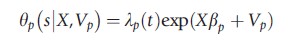
If the no-anticipation assumption holds, the ex-post effect of treatment δ can be specified within the MPH rate model for exits from the state

In this specification s describes the start of treatment and the indicator function I(t>s) denotes if after t units of time the individual is exposed to the treatment. The key problem in the estimation is that the timing of the start of treatment s is often not independent of unobserved characteristics V. Therefore, the treatment effects model is extended by a PH rate model for the start of treatment

By allowing the unobserved terms in both hazard rates to be dependent, the model allows for endogeneity of the start of treatment. This model is often referred to as timing-of-events model.

To estimate the timing-of-events model, maximum likelihood estimation should be used. This requires the specification of the baseline hazards λ_e(t) and λ_p(t), as well as the joint distribution of the unobserved heterogeneity terms V_e and V_p. The model can allow for heterogeneous treatment effects. In particular, the treatment effect d can be made dependent on observed characteristics X, unobserved characteristics V, the elapsed duration in the state t, the moment of starting treatment s, and thus also on the elapsed duration since the start of the treatment t-s.

This timing-of-events approach has in dynamic settings a number of advantages over other methods for treatment evaluation. Most important is that if treatment starts at some moment during a spell, it is difficult to define control groups for those individuals who receive treatment. In many cases, all individuals will receive treatment at some point when staying sufficiently long in the state. Therefore, individuals who are observed to be untreated are often so because they left the state relatively fast. Next, the timing-of-events model allows for selection on unobservables. Furthermore, most alternative methods require discretizing time, which has the disadvantage that results might be sensitive to the choice of the unit of time. Finally, the timing-of-events model explicitly models dynamic selection and the entry into treatment, which might be of interest in itself.

References:

1. Heckman, J. J. and Singer, B. (1984). A method for minimizing the impact of distributional assumptions in econometric models for duration data. Econometrica 52, 271–320.
2. Abbring, J. H. and van den Berg, G. J. (2003). The non-parametric identification of treatment effects in duration models. Econometrica 71, 1491–1517.
3. Abbring, J. H. and van den Berg G. J. (2005). Social experiments and instrumental variables with duration outcomes. Discussion Papers 05–047/3. Amsterdam: Tinbergen Institute.
4. Abbring, J. H. and Heckman, J. J. (2007). Econometric evaluation of social programs, part III: Distributional treatment effects, dynamic treatment effects and dynamic discrete choice, and general equilibrium policy evaluation. In Heckman, J. J. and Leamer, E. (eds.) Handbook of econometrics, vol. 6B. Amsterdam: Elsevier Science.
5. Breslow, N. (1974). Covariance analysis of censored survival data. Biometrics 30, 89–99.
6. Cox, D. R. (1972). Regression models and life tables. Journal of the Royal Statistical Society Series B 34, 187–220.
7. Cox, D. R. (1975). Partial likelihood. Biometrika 62, 269–276.
8. Ham, J. C. and Rea, S. A. (1986). Unemployment insurance and male unemployment duration in Canada. Journal of Labor Economics 5, 325–353.
9. Han, A. K. and Hausman, J. A. (1990). Flexible parametric estimation of duration and competing risk models. Journal of Applied Econometrics 5, 1–28.
10. Kalbfleisch, J. D. and Prentice, R. L. (1980). The statistical analysis of failure time data. New York: Wiley.
11. Kaplan, E. L. and Meier, P. (1958). Nonparametric estimation from incomplete observations. Journal of the American Statistical Association 53, 457–481.
12. Lancaster, T. (1990). The econometric analysis of transition data. Cambridge: Cambridge University Press.
13. Ridder, G. (1984). The distribution of single-spell duration data. In Neumann, G. R. and Westergard-Nielsen, N. C. (eds.) Studies in labor market dynamics. Berlin: Springer.
14. Ridder, G. (1987). The sensitivity of duration models to misspecified unobserved heterogeneity and duration dependence. Mimeo.
15. Ridder, G. and Tunali, I. (1999). Stratified partial likelihood estimation. Journal of Econometrics 92, 193–232.
16. Salant, S. (1977). Search theory and duration data: A theory of sorts. Quarterly Journal of Economics 91, 39–57.
17. Van den Berg, G. J. (2001). Duration models: Specification, identification, and multiple duration. In Heckman, J. J. and Leamer, E. E. (eds.) Handbook of econometrics, vol. 5. Amsterdam: North Holland.
18. Van der Klaauw, B. and Wang, L. (2011). Child mortality in rural India. Journal of Population Economics 24, 601–628.