Models for Discrete Choice Models

This article will survey the application of discrete choice models in health economics. The application of econometrics to understanding the health system takes place at several levels:

• Aggregate: modeling the behavior over time of aggregates such as health care spending and demographics.
• Market: modeling the behavior of specific markets such as hospital services markets and market structures and labor markets such as the market for nurses.
• Individual: modeling the behavior of individuals making decisions such as whether to have insurance, visit a physician, or how intensively to use the health care system.

It would be overly ambitious to attempt to cover the field in a single essay. This survey will focus on the third topic. The analysis of individual behavior in health economics generally involves a particular style and tradition of econometric model building. At the individual level, behavior often takes the form of discrete choices over particular sets of alternatives. To focus ideas, we consider the examples of whether individuals purchase insurance or not, or how they report their health status or satisfaction, or which type of products to purchase, or how many times they visit the physician or engage in a particular behavior such as smoking or consuming narcotics. Each of these is a discrete choice, in most cases, a binary choice between two distinct alternatives. Understanding these individual choices helps the analyst to understand aggregate behavior and, for example, the impact of policy changes on behavior.

Choice Modeling: Theory And Econometrics

There are two fundamental building blocks that underlie the methodology of discrete choice modeling, the model of random utility and the basic econometric binary choice model for choice between two alternatives. (The theory of random utility began in the 1920s. It gained great momentum with the econometric research by McFadden, 1974.) The econometric approach to analyze discrete choices departs from the assumption that an individual’s behavior reflects an underlying preference structure that is consistent with the familiar constructs of microeconomic theory. That is, the individual’s preference are continuous, complete, and transitive. The implication is that choices are made in the setting of a particular process, or calculus. The nature of the choice mechanism, if not the choice itself, follows from some familiar axioms of economic theory: choices are continuous, meaning that small variations in circumstances generally lead to small or no changes in decisions; choices are complete, meaning that decision makers are able to rank any pair of alternatives presented; and choices are transitive, meaning that, in broad terms, choices are logically consistent. The model builder moves forward from this underlying preference structure to a model of the value or utility of a specific alternative, which it is convenient to label U_ij, with U meaning utility and j indicating the alternative. Thus, U_ij is the utility, or value to individual i of making choice j. The centerpiece of the econometric model is the random utility model (RUM), which states that from the point of the model builder, U_ij is a random variable with a particular form that will be described. It is noted at this convenient juncture, that the idea of random utility is from the point of the observer. It does not imply that individuals make decisions randomly, for example, by using a coin toss to decide whether or not to visit a physician or to consume a narcotic. The random utility model is used as a platform for the analysis on which aspects of behavior are ‘observable’ (or nonrandom), whereas others are ‘unobservable’ (so, from the observer’s standpoint, random). Thus, for example, it can be confidently said that price is a determinant of whether an individual chooses to smoke. But, there are also other intrinsic and inherently unobservable features of the individual’s psyche that motivate a decision to smoke; price alone is not the full story. The observed outcome appears random because observable information is not sufficient to provide a complete explanation of the observed choice.

Random Utility

For convenience, it will help to write the RUM in a particular additive form,

The model of random utility is stated from the point of view of the analyst – it embodies their understanding of individual behavior. It states that the utility of the observed individual is composed of a deterministic part that is amenable to model building and responds predictably to observable stimuli, and a random part that embodies the unobservable aspects of individual preference. It is crucial to the understanding of behavior that it is assumed that under the same circumstances, the individual will always behave the same way. The randomness of random utility describes the analyst’s understanding of the differences across different people.

It should also be noted that RUM is a model – a description of behavior. A common mistake is to attack the RUM as if it was an immutable statement of the precise nature of underlying utility, which would then be characterized as hopelessly naıve. The RUM is a broad characterization of the process that lies behind observations of choices that individuals make. To make it convenient to discuss ideas, a particular form for the utility function is assumed,

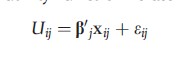
For the less mathematically inclined reader, it is noted, the vector symbol b`x is used here as a shorthand for the equivalent linear equation, U_ij=β₀+β₁x_ij1+ β₂x_ij2+….β_Kx_ijK+ ε_ij. The variables x_ijk represent either attributes of the choices, such as the price of a particular kind of insurance policy, or characteristics of the individual, such as age, gender, or income. The definition of a utility function in this form embodies the assumption that these features influence the choice made because they influence utility. For example, an increase in the price of an insurance plan (it is assumed) will make that plan less desirable – the choice of that plan, all else equal, will afford the individual lower utility (because the plan’s greater price will divert income from other activities that would provide utility). The lower utility, working a step backward, makes it less likely that an individual would choose that plan instead of others available.

Binary Choice

The second fundamental building block of a paradigm of modeling discrete choices is a mechanism that translates unobserved utility into an observed counterpart. The departure point is the choice between two alternatives. The random utilities for two alternatives, for example, ‘being a smoker,’ or ‘being a nonsmoker,’ would be represented by

These two utility functions are implied by the RUM. The assumption that observed behavior is consistent with an underlying preference structure of utility maximization implies that the (now hypothetical) individual i will make choice S if U_iS>U_iN and will make choice N if U_iN>U_iS. Thus, the decision actually made is termed the revealed preference – the decision to be a nonsmoker reveals that the individual prefers being a nonsmoker to being a smoker. (There is a slightly inconvenient ambiguity in how to break a tie. It is assumed that if the individual is indifferent between the two alternatives, they will choose alternative N (or, the first alternative). In more formal mathematical terms, since the random variables involved are continuous, the probability of a tie is zero and one need not worry about it in developing the theory. It might be tempting to think the individual mentally tosses a coin when faced with indifference between two choices. However, this would violate the continuity assumption made earlier, and seems unrealistic as well.)

The utility maximization assumption implies an econometric model: Specifically, it can be reasoned backwards from the observed choice to the underlying outcome. In our example,

Collecting terms, this implies that if choice N is made, then it follows that (β`<sub>N</sub>x<sub>iN</sub>-β`_Sx_iS) +(ε_iN-ε_iS)≥0. Combining and renaming terms, it is determined that choice N will be made if y`x_i +ε_i≥0. This provides the underpinning of an econometric model that will help in understanding individual choices and the differences across individuals. In particular, if two individuals who make different choices are observed, two underlying sources for the difference can be asserted. The first arises from the deterministic parts of the utility functions. The second comes from the random parts. Suppose, for example, that income is the only observable difference between individuals in the analysis, income appears in the deterministic part of the utility functions. Then, according to the model, if income is higher, it makes one of the two choices more likely and the other less so. Of course, this does not imply that it can be deduced which choice the individual makes. The presence of the random term in the model implies that the information in hand suggests the impact of changes in income will be exerted only on the probabilities. Therefore, implications of the model can only be drawn in probabilistic terms. The model is completed with a specification of the probability distribution of the random term. Traditionally, the analysis has been based on one of two frameworks. The most appropriate choice for the behavior of ε would seem to be motivated by the central limit theorem, which describes the behavior of aggregates of small influences. Assuming a normal distribution produces the probit model. Although less natural from a behavioral standpoint, because of its convenient mathematical properties, the logistic distribution has often been specified instead. This gives rise to the logit model of binary choice. (Foundational work on this specific type of model appears in the bioassay literature. The modern, social science paradigm can be traced back to work on information theory by Walker and Duncan (1967). An introduction to the use of binary choice models is contained in Greene and Hensher (2010).)

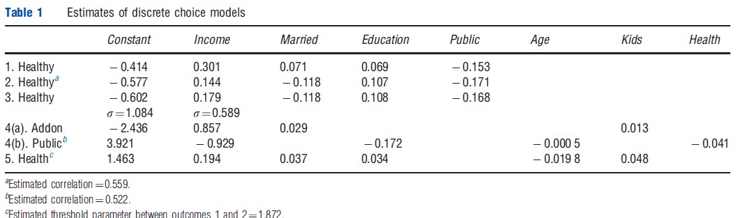
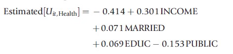
Before turning to a survey of extensions, an application that should help to focus ideas is noted. Riphahn, Wambach and Million (RWM, 2003 – Riphahn et al., 2003) studied the use of the health care system by a large sample of German households. Among the interesting variables in their data set is a question about health satisfaction (HSAT), a scale variable coded 0 to 10. For purposes of the application, this variable is recoded to be HEALTHY=0 if HSAT<6 and HEALTHY=1 if HSAT>6. The average of HSAT in the sample is 6.8. (This sample is a panel. There are 27 326 household years in the data, but the sample is 7293 households.) The RWM data is used to construct a probit RUM of the binary choice of whether the individual reported feeling healthier than average or not. Note that it is not appropriate to assume that the individual reports that they feel healthier than the average person in the sample – they would obviously not know that. An ongoing theme in this area of research is an understanding of how the model should accommodate the idea that different individuals would view the term ‘healthy’ differently. If there were an objective construct, ‘health,’ different individuals at the same location on the scale might still report different answers. The estimated equation shown in the first row of Table 1 is

MARRIED and PUBLIC are dummy variables for marital status and whether the individual purchased public health insurance (roughly 88% of people did). (How coefficients in a probit model are computed, what they mean, and how they are used for estimation and inference in an analysis is discussed in Greene (2011, chapter 17) and in Greene and Hensher (2010).) Based on the description so far, one would infer from these results that increases in income, and education, and if one is married, all act to make it more likely that an individual will report feeling healthy, whereas if they purchased public insurance, they are more likely to report feeling unhealthy. An important point to note – will be returned to it below – is the possibility that the purchase of insurance included in this equation is, itself, motivated by the individual’s health satisfaction. This ambiguous directionality of the causal effect in this equation is a fundamental aspect of the model building effort. (The opportunity to discuss elements of the econometric/ statistical framework related to the estimation machinery – parametric vs. nonparametric, Bayesian vs. Classical, etc. – is not used. Although they are important questions, they are only secondary to the focus on the paradigm itself. See Greene (2011) for further discussion.)

Issues In Binary Choice Modeling

The binary choice model can be used to understand individual behavior or to try to forecast it. For example, in the preceding model, it is found that INCOME seems to be an important variable – its coefficient is very large compared to the others. Translating the coefficients in the model into meaningful quantities is one of the burdens of the model builder (see Greene (2011)). There are also some fundamental issues that are relevant here and in other modeling contexts described later. Several of them are noted, in particular: endogeneity, heterogeneity (and panel data) and selectivity. It will be convenient to pivot this discussion off the small model given above in the section on Extended Choice Models.

• The model for HEALTHY includes INCOME. It might be supposed that a self-report of healthy is a revelation of an underlying, objective measure of health outcome – an individual who reports that they feel healthy really is healthier than one who does not. It may well be that one’s health is a determinant of their ability to earn their income, so that if a causal effect can be considered between healthy and income in the equation, it runs in both directions. That would require some special treatment in estimation of the model. Likewise, the model seems to suggest that those who purchase public health insurance feel less healthy. It is possible that individuals who feel less healthy (because they are less healthy) are more likely to purchase the insurance. Once again, the direction of the causality is uncertain. This problem of endogeneity (of the explanatory variable) is common in the analysis of health-related outcomes.
• It is difficult to argue that the model builder should ignore the heterogeneity issue. With panel data such as available here, there are a variety of strategies that can be used. The general result is that if there are features of the individual, albeit unobservable by the analyst, that can be reasonably assumed to be constant through the time period for which the data are observed, then, with some defensible assumptions, the model can be enhanced to accommodate individual heterogeneity. The ‘random effects’ (RE) model is an example. In this framework, the random component of the random utility model is assumed to include two parts, the overall random term, ε_ijt that contains the effects that vary from period to period, and a time constant term, u_ij that is a fixed (albeit unobserved) characteristic of the individual. The RE model assumes that this effect can be modelled as a random variable that varies across individuals. Row 2 of Table 1 shows estimates of the same model shown earlier, but with a common random effect included in the equation. The estimate of p of 0.559 is a measure of the variation of the time invariant part of the random part of the utility function. To assess how important this term is, the variance of this term is computed, which is p/(1- p)=1.267. The model assumes that the variance of e is 1.000, so it would appear that there is greater variation in the invariant unobserved effect than in the time variant part.
• The model contains a coefficient of 0.301 on income. However, this value is translated into a meaningful measure of causal influence of income on health satisfaction, and will be translated into the same measure for every individual in the sample. This seems naıve – the impact of income on the probability of reporting good health will surely differ from one individual to the next. Although it has already been acknowledged that the model is meant to be succinct and descriptive, this still seems like a degree of realism that would prove important to consider. How one should accommodate heterogeneity in a choice model that is an econometric issue which many authors have considered (see, e.g., Train, 2003). An extension of the RE model is a similar model that allows the marginal utilities to vary over individuals as well. The random parameters model (RPM) allows coefficients to have a distribution across individuals. Row 3 of Table 1 shows the estimates of a model with random coefficients. It requires a bit more work to translate the estimates of the structural parameters of an RPM into a meaningful set of numerical results. It can be seen in Table 1 that in the distribution of income coefficients across the sample individuals, it appears that the standard deviation is much greater than the mean.
• Data on health outcomes are often self reported. When the sample, itself, is self selected, then the generality of the econometric model is called into question. In particular, when individuals select themselves into the sample, and the motivation for participation is connected to the health outcome being analyzed, a problem of sample selection arises. Studies of drug efficacy based on data gathered from physician visits would present an example. Jones (2007) describes some methods of analyzing models with sample selection. Some general commentary on application of the models in health economics is given in Madden (2008).

Extended Choice Models

The binary choice model based on a random utility platform with a linear index function is the workhorse of discrete choice modeling in health econometrics. There are a wide range of variations on the binary choice model that accommodate different sampling frameworks and decision situations. Madden (2008), for example, discusses the choice of sample selection versus two part models. Broadly, two part models examine consumer decisions as a pair of sequential decisions. For example, in Harris and Zhao (2007), the authors examined smoking behavior. A two part model of the intensity of smoking behavior (e.g., number of packs of cigarettes per week) might involve a decision of whether or not to be a smoker, then, for smokers, a second decision, how much to smoke. The core of the model is its allowance of the determinants of the two decisions to differ – for example, price might motivate the intensity variable, but might be tangential to the base decision whether to be a smoker or not. For another example, another interesting variable in the RWM study is ADDON, which is an indicator of whether the observed individual purchased an enhanced type of health insurance. To purchase the addon insurance, one must purchase the public insurance, so a model that purports to describe ADDON must account for the condition that the individual purchases the public insurance. Not all individuals did; approximately 88% of the individuals purchased the public insurance. The model then describes these two simultaneous decisions. Row 4 of Table 1 contains estimates of such a model. The fairly high value of the correlation coefficient is interpreted to suggest that the unobserved factors that determine purchase of the public insurance also help to explain purchase of the addon insurance.

The list of similar extensions of the basic binary choice model is extensive. Two major directions of research in discrete choice modeling are examined, ordered choice and unordered choice.

Ordered Choices

The example of modeling in health economics includes a variable HSAT, which is self-reported health satisfaction. In the original data, this variable is coded 0,1, …, 10. That is, it is a ‘scale’ variable coded on an 11-point scale. Many surveys, such as the British Household Panel Survey (BHPS – see Contoyannis et al., 2004) and the German Socioeconomic Panel (GSOEP – see RWM (2003)) that have been used above, include attitude variables such as health satisfaction (HSAT) or subjective well being (SWB). Pudney and Shields (2000) examine the promotion process in the UK nursing market. Conventional regression methods are inappropriate for modeling such variables. A natural extension of the random utility model provides an appropriate framework for the analysis. The model supposes that the observed scale variable reflects an underlying continuous preference scale. Thus, in the RUM framework, it begins with an assumption that U_i,health= β`x+ε as usual. The observed outcome is not utility, or the continuous counterpart to ‘health.’ Rather, the respondent is given an opportunity to place themselves in their choice on a scale, indicated ‘0’, ‘1’, etc. The outcomes are thus indicators of the strength feeling on the utility scale. For the 0–10 scale, for an individual in particular, a choice of 8 rather than 7 indicates an increase in perceived health, but the difference of one unit is not meaningful. Thus, the difference between 8 and 7 of 1 is not necessarily the same as the difference between 6 and 5. The observed outcome only suggests that a response of 8 represents a greater value on the preference scale than a 7 would. This observation mechanism gives rise to an ordered choice model. The ordered choice model has proved useful for many applications in health economics (and many other fields). See Greene and Hensher (2010) for an extensive survey. See Boes and Winkelmann (2004, 2006), and Contoyannis et al. (2004) for applications.

Like the binary choice model, the ordered choice model has been extended in many directions. For example, Harris and Zhao (2007) examined data on tobacco use behavior in which there is reason to suspect willful misreporting. The accommodation in the ordered choice model is to ‘inflate’ the zero outcome. An interesting problem in understanding ordered choices is that the model assumes that all individuals interpret the scaling in the same way. This is likely to be particularly problematic when models are used to compare health outcomes across cultures and countries. In the simple example above in the section on Binary Choice, the model is likely to produce different predictions if it is used to compare two countries in which one is populated by inherently optimistic individuals whereas the other is less so. The meaning of ‘middling health’ might be very different in the two cases, being a very negative statement in the first case noted and a positive one in the second. King et al. (2004) and a succession of authors have designed models that involve anchoring vignettes. Vignettes are designed to solicit attitudes on scales that (arguably) all respondents should agree on. The scale built into the ordered choice model is calibrated to accommodate these differences in the arrangement of the outcomes on the preference scale. King et al.’s. study used the approach to compare survey data on political efficacy in Mexico and China.

Unordered Choices

Models of discrete choice are also extended to analyze situations in which individuals select among unordered alternatives. For example, modeling a choice among different health insurance plans is considered. To construct an application, it supposes that plans are differentiated by features such the amount of the copayment, ceiling, and coverage of specific situations and by the price of the insurance plan. An RUM of the choice of which plan to choose would assign a utility to each plan:

Maintaining the assumption of utility maximization, it is assumed that the individual makes the choice that provides the greatest utility. Because it is a RUM, as in the previous cases, the model is completed by specification of the random terms. The counterpart to the binary probit model in this setting is the multinomial logit model (MNL). Since the work of McFadden (1974), the MNL has been used by generations of researchers to model unordered choices among multiple alternatives. An example is Gertler et al. (1987) who analyzed a Peruvian household survey of the choice of health care provider, public clinic, public hospital, or private doctor. The focus of extensive recent research has been on formulating more realistic formulations of the choice model that accommodate heterogeneity in preference structures. A leading example is Fiebig et al.’s (2010) development of a generalized mixed logit model, which is an elaborate form of random parameters model.

Multinomial logit models and variants such as the mixed logit model provide information on the preference structure and on effects of interest such as how price influences the choice among the alternatives. Another useful quantity revealed through the estimated preference structure is willingness to pay. It can be recalled, the model does not predict utilities – there is an inherent scaling and translation problem. But, the model does provide information about marginal utilities. The standard measure of willingness to pay for an attribute of a choice in a multinomial choice context is

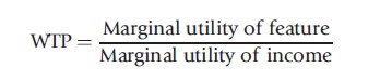
In this example, the marginal willingness to pay measure for an increase in the limit of the dental coverage of our (hypothetical) policy would be WTP_dental=β_D/y. This would provide an empirical estimate of the amount that an individual would value (i.e., be willing to pay) for an increase in the desirable attribute of the choice, such as an increase in the amount of dental coverage in our example.

Conclusions

The econometric models examined in this essay form the platform for a large share of the empirical analysis of individual behavior in health economics. The random utility model and its corollary, the fundamental model of binary choice, are the pillars of econometric analysis throughout the social sciences. Because the choice variables in health economics often involve Likert-like scales and choices among sets of alternatives, the ordered choice and unordered choice models are natural settings in which to examine health economics outcomes.

References:

1. Boes, S. and Winkelmann, R. (2004). Income and happiness: New results from generalized threshold and sequential models, vol. 1175, SOI Working Paper 0407, IZA Discussion Paper, IZA.
2. Boes, S. and Winkelmann, R. (2006). The effect of income on positive and negative subjective well-being. University of Zurich, Socioeconomic Institute, Discussion Paper 1175, IZA.
3. Contoyannis, A., Jones, A. and Rice, N. (2004). The Dynamics of Health in the British Household Panel Survey. Journal of Applied Econometrics 19, 473–503.
4. Fiebig, D., Keane, M., Louviere, J. and Wasi, N. (2010). The generalized multinomial logit model: Accounting for scale and coefficient heterogeneity. Marketing Science 29, 393–421.
5. Gertler, P., Locay, L. and Sanderson, W. (1987). Are user fees regressive? The welfare implications of health care financing proposals in Peru. Journal of Econometrics 36, 67–88.
6. Greene, W. (2011). Econometric analysis. Englewood Cliffs, NJ: Prentice Hall.
7. Greene, W. and Hensher, D. (2010). Modeling ordered choices. Cambridge: Cambridge University Press.
8. Harris, M. and Zhao, X. (2007). Modeling tobacco consumption with a zero inflated ordered probit model. Journal of Econometrics 141, 1073–1099.
9. King, G., Murray, C., Salomon, J. and Tandon, A. (2004). Enhancing the validity and cross cultural comparability of measurement in survey research. American Political Science Review 98, 191–207.
10. Madden, D. (2008). Sample selection versus two part models revisited: The case of female smoking and drinking. Health Economics 27, 300–307.
11. McFadden, D. (1974). Conditional logit analysis of qualitative choice behavior. In Zarembka, P. (ed.) Frontiers in econometrics. New York: Academic Press.
12. Pudney, S. and Shields, M. (2000). Gender, race, pay and promotion in the British nursing profession; estimation of a generalized ordered probit model. Journal of Applied Econometrics 15, 367–399.
13. Riphahn, R., Wambach, A. and Million, A. (2003). Incentive effects on the demand for health care: A bivariate panel count data estimation. Journal of Applied Econometrics 18, 387–405.
14. Train, K. (2003). Discrete choice methods with simulation. Cambridge: Cambridge University Press.
15. Walker, S. and Duncan, D. (1967). Estimation of the probability of an event as a function of several variables. Biometrika 54, 167–179.