Models for Count Data

Count data regression is now a well-established tool in econometrics. If the outcome variable is measured as a non-negative count, y, yϵN₀₌ 0, 1, 2,…. and the object of interest is the marginal impact of a change in the variable x on the regression function E[y|x], then a count regression is a relevant tool of analysis. Fully parametric formulations of count models accommodate this discreteness property of the distribution, with probability mass at nonnegative integer values only. By contrast, some semiparametric regression models accommodate only nonnegativity but not discreteness. For such data, a linear regression is generally not efficient, and hence the standard count model is a nonlinear regression. A fully parametric formulation is more attractive if the researcher’s interest is in the full distribution of the data, whereas a semiparametric model like nonlinear least squares is often used when the focus is on the conditional mean only.

Cross-section and panel data on event counts, for example, doctor visits, hospital admissions, and many measures of health-care utilization, are very common in empirical health economics. This has contributed to the use of count data regressions. This article covers the case where all regressors are exogenous or predetermined. The empirically important case in which some regressors are endogenous is treated in other articles. The focus here is on classical inference, but all models considered here are amenable to Bayesian analysis.

Poisson Regression

The starting point of many count data analyses is the Poisson regression, derived from the Poisson distribution, for the number of occurrences of the event, with probability mass function

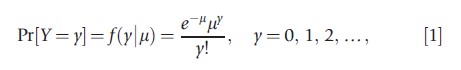
where μ is the intensity or rate parameter. The first two moments of this distribution, denoted P[μ], are E[Y]=μ, and V[Y]=μ, which is the well-known equidispersion property of the Poisson distribution. The Poisson regression results from the parameterization μ=μ(x), where x is a K-dimensional vector of exogenous regressors. The usual specification of the conditional mean is

Standard estimation methods are fully parametric Poisson maximum likelihood (PML), ‘semiparametric’ methods such as nonlinear least squares, or (weighted) moment-based estimation, based on the moment condition E[y-exp(x`β)|x]=0 possibly further augmented by the equidispersion restriction used to generate a weighted moment function.

According to standard maximum likelihood theory, if the Poisson model is parametrically correctly specified, the maximum likelihood estimator (MLE) β_p is consistent for β, with covariance matrix estimated by

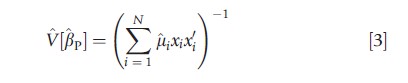
where μ_i=exp(x`_iβ_p). The use of this formula can be misleading if the equidispersion assumption is incorrect.

The Poisson regression is founded in the Poisson point process for the occurrence of the event of interest. This process is a characterization of complete randomness, which excludes any form of dependence between events, either cross sectionally or over time, and any form of nonstationarity. In the Poisson regression, these assumptions are conditional on the covariates xi, which reduces the restrictiveness of the model. Even when analysis is restricted to cross-section data with strictly exogenous regressors, the basic Poisson regression is restrictive for most empirical work. First, the mean-variance equality restriction will be violated if there is significant unobserved heterogeneity in cross-section data – in which case (conditional) variance will exceed (conditional) mean. This feature, referred to as overdispersion (relative to the Poisson), manifests itself in a variety of data features, most noteworthy being the excess zeros problem.

Overdispersion

Overdispersion results from many different sources and is consistent with a variety of different deficiencies of the Poisson regression, including serial dependence, spatial dependence, or contemporaneous dependence of events. This motivates replacing the Poisson distribution with more flexible functional forms that can accommodate overdispersion as well as its other specific limitations.Thus, many functional forms are generated as Poisson mixtures. Replace the parameter μ_i in (1) by μ_iv_i, where v_i represents individual-specific, independently and continuously distributed, separable unobserved heterogeneity. Next make an assumption about the distribution of vi Finally, derive a new functional form by integrating out v (subscript omitted) – a mathematical operation equivalent to averaging with respect to the assumed distribution of v. A shortcut is to start with the more flexible functional form (i.e., the mixture distribution) without going through the intermediate mathematical step.

Provided the conditional mean is correctly specified, the PML estimator (PMLE) is consistent but not efficient in the presence of overdispersion. Considering overdispersion, one can use the pseudo-ML or quasi-ML approach, again using the PMLE for point estimates but computing the (Eicker– White) robust estimate of the variance–covariance matrix using an expression of the form V_Rob[β_p]=A^-1BA^-1 where A=∑^N_i=1μ_ix_ix<sub>i`</sub>and B=∑<sup>N</sup><sub>i=1</sub>(y<sub>i</sub>-μ<sub>i</sub>)<sup>2</sup>x<sub>i</sub>x<sub>i</sub>` and μ_i=exp(x_i`β_p), that is, the point estimates of β are as in pseudo-ML theory, but its sample variance is obtained robustly.

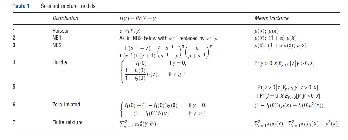
Efficient estimation of overdispersed model is possible if more specific parametric assumptions are invoked. The negative binomial (NB) regression is an example of a mixture model. It can be derived as a Poisson–Gamma mixture. Given the Poisson distribution f(y|x,v)=exp(-μv)(μv)^y/y! with the mean E[y|x,v] = μ(x)v, v>0, where the random variable v represents multiplicative unobserved heterogeneity, a latent variable assumed to be independent and separable has Gamma density g(v)=v^a-1exp(-v)/Г(a), with E[v]=1 and variance a (a>0). The resulting mixture distribution is the NB2 (negative binomial with quadratic variance), which has mean E[y|x]= μ(x)] and variance V[y|x]= [1+aμ(x)]μ(x)>E[y|x], thus accommodating overdispersion. Relative to the Poisson, the overdispersed distributions have more probability mass at zero and high values of y. The same approach can be used with other mixing distributions.The NB1 variant of the NB, which has variance linear in μ(x), and the Poisson–lognormal mixture are two popular alternatives to the Poisson. The formulae for the probability mass function of NB1 and NB2 distributions are shown in Table 1.

Test Of Overdispersion

The null hypothesis of equidispersion can be tested by postulating an alternative overdispersed model. A formal test of the V[y|x] = E[y|x] property can be based on the equation

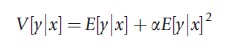
which is the variance function for the NB1 model. Equivalently, H₀:a= 0 against H₁:a>0 is tested.

The test can be implemented by auxiliary regression of the generated dependent variable ((y-μ)²-y)/μ on μ, without an intercept term, and performing a t test of whether the coefficient of μ is 0. However, the rejection of the null does not automatically indicate a suitable alternative model because that outcome is consistent with failure of the null model in many different ways.

Alternatives To The Poisson

The NB regression has been found to fit well many types of data, including those with ‘excess zeros.’ It has an analytical closed form. Functional forms resulting from other mixing assumptions, for example, the lognormal, often do not have a closed form, although estimation using either simulationbased methods or quadrature methods for numerical integration is straightforward to implement.

The classic gamma heterogeneity assumption underlying NB2 is somewhat special. Modern approaches, however, can handle more flexible models where the latent variables are nonseparable, which means that in principle unobserved heterogeneity impacts the entire distribution of the outcome of interest. Quantile regression and finite mixtures are two examples of such nonseparable models.

The literature on new functional forms to handle overdispersion is large and still growing. Despite the availability of many functional forms, a relatively small class of models has attained much popularity in health econometrics. This includes especially the NB regression (NBR) presented above, the two-part model (TPM) or the hurdle model, and the zeroinflated Poisson (ZIP) and zero-inflated NB (ZINB), which collectively dominate the applied literature and form the set of basic parametric count regression models. These models are all mixtures of Poisson-type models. Discussion of these models provided as follows.

Hurdle Model

The hurdle model or TPM relaxes the assumption that the zeros and the positives come from the same data generating process. The zeros are determined by the density f₁(·), so that Pr[y=0]= f₁(0) and Pr[y>0]=1-f₁(0). The positive counts come from the truncated density f₂(y|y>0)=f₂(y)/(1-f₂(0)), that is multiplied by Pr[y>0] to ensure that probabilities sum to 1. Thus, suppressing regressors for notational simplicity,

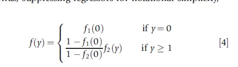
This specializes to the standard model only if f₁(·)=f₂(·). This model can handle both excess zeros and too few zeros.

A hurdle model has the interpretation that it reflects a two-stage decision-making process, each part being a model of one decision. The two parts of the model are functionally independent. Therefore, ML estimation of the hurdle model can be achieved by separately maximizing the two terms in the likelihood: one corresponding to the zeros and the other to the positives. A binary outcome model is used to model the positive outcome and a truncated Poisson or NB for the second part. The first part uses the full sample, but the second part uses only the positive-count observations.

For certain types of activities, such a specification is easy to rationalize. For example, in a model that explains the number of packs of cigarettes smoked per day, the survey may include both smokers and nonsmokers. The first part of the hurdle model determines whether or not one smokes and the second part determines the intensity, i.e., the number of packs smoked, given that at least one pack is smoked.

Models For Zero-Inflated Data

The zero-inflated model was originally proposed in manufacturing quality control settings to handle data with excess zeros relative to the Poisson. Like the hurdle model, it supplements a count density f₂(·) with a binary process with density f₁(·). If the binary process takes value 0, with probability f₁(0) then y=0. If the binary process takes value 1, with probability f₁(1), then y takes count values 0,1,2,… from the count density f₂(·). This lets zero counts occur in two ways: as a realization of the binary process and as a realization of the count process when the binary random variable takes value 1.

Suppressing regressors for notational simplicity, the zero-inflated model has density

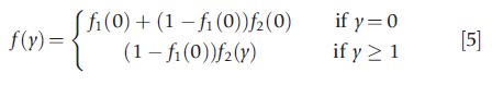
As in the case of the hurdle model, the probability f₁(0) may be a constant or may be parametrized through a binomial model like the logit or probit to capture dependence on observable factors. Once again, the set of variables in the f₁(·) density need not be the same as those in the f₂(·) density. However, identifying the separate roles of factors that affect f₁(0) and f₂(y) is generally challenging.

Finite Mixture Models

The NB model is an example of a continuous mixture model. An alternative approach uses a discrete representation of unobserved heterogeneity to generate a class of models called finite mixture models (FMM) – a particular subclass of latent class models.

An FMM specifies that the density of y is a linear combination of m different densities, not necessarily from the same parametric class, where the jth density is f_j(y|β_j), j=1, 2, …, m. Thus an m-component finite mixture is

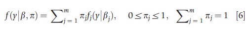
For example, a two-component (m = 2) mixture of f₁(y|x,β₁) and f1(y|x,β₂) may reflect the possibility that the sampled population contains two ‘types’ of cases, whose y outcomes are characterized by distributions with different moments. The mixing fraction π₁ is, in general, an unknown parameter which could, for additional flexibility, be parameterized in terms of observed variable(s) z.

The FMM specification is attractive for empirical work in cross-section analysis because its functional form is flexible. Mixture components may come from different parametric families, although commonly they are specified to come from the same family. The mixture components permit differences in conditional moments of the component distributions, and hence in the marginal effects. In an actual empirical setting, the latent classes often have a convenient interpretation in terms of the differences between the underlying subpopulations. However, the number of latent classes is generally unknown and has to be treated as an additional parameter. This is a nontrivial complication that has often been handled as a model selection problem that is solved using penalized likelihood criteria. Bayesian analyses using Dirichlet process mixtures potentially allow for additional flexibility.

The main features of some popular models are summarized in Table 1.

Quantile Regression For Counts

Quantile conditional regression (QCR) is a robust semiparametric methodology for continuous response data. The conditional quantile function is a more general object of interest than the traditional conditional mean because it allows us to study potentially different responses in different quantiles of the outcome variable, and thus the entire distribution. It is consistent under weak stochastic assumptions and is equivariant to monotone transformations of the outcome variable. It is attractive because it potentially allows for response heterogeneity at different conditional quantiles of the variables of interest. By extending it to count data regression, one can overcome the standard and restrictive models of unobserved heterogeneity based on strong distributional assumptions. Further, QCR permits the study of the impact of regressors on both the location and scale parameters of the model and thus supports a richer interpretation under weaker distributional assumptions. A difficulty arises because the quantiles of discrete variables are not unique as the cumulative distribution function is discontinuous with discrete jumps between flat sections. By convention, the lower boundary of the interval defines the quantile in such a case. However, recent theoretical advances have extended QCR to a special case of count regression.

The key step in the extension of QCR to counts involves replacing the discrete count outcome y with a continuous variable z =h(y), where h(·) is a smooth continuous transformation. The standard linear QCR methods are then applied to z. The particular continuation transformation used is z=y+u, where u~U[0,1] is a pseudorandom draw from the uniform distribution on (0,1). This step is called ‘jittering’ the count. Point and interval estimates are then retransformed to the original y-scale, using functions that preserve the quantile properties.

Panel Data

Count data panel models, like their linear counterparts, use three main frameworks: population-averaged (PA) models, random-effect (RE) models, and fixed-effect (FE) models. All are widely used in health econometrics. Maximum likelihood as well as moment-based estimation is common.

Given the scalar dependent variable y_it with vector of regressors x_it where i, i=1,…,N, denotes the individual and t (t=1,…,T) denotes time, the case of ‘short panel’ (small T) is empirically in health applications.

Many complications of count data panel models stem from discreteness of y and nonlinearity of the conditional mean. Assume multiplicative individual-specific scale effect a_i applied to exponential function,

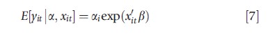
As x_it includes an intercept, a_i may be interpreted as a deviation from 1 because E(a_i|x)=1.

Pooled Or Population-Averaged Models

Operationally speaking, pooling involves ‘stacking’ cross-section observations and applying cross-section methods. Pooling multiple cross-section involves a strong assumption. The observations y_it|a_i, x_it are treated as independent, after assuming a_i= a, which implies absence of unobserved heterogeneity. The pooled model is also called the PA model. For parametric models, it is assumed that the marginal density for a single (i, t) pair,

is correctly specified, regardless of the (unspecified) form of the joint density f(y_it,…,y_iT|x_il,…,x_iT,β,g). The PA specification accommodates some assumption about conditional dependence between y, over both i and t. Serial correlation of y suggests conditional dependence. Hence, after estimating the pooled model (by ML or moment-based estimator such as nonlinear least squares), ‘residuals’ may be dependent; hence a panel-robust or cluster-robust (with clustering on i) estimator of the covariance matrix can then be applied to adjust standard errors for such dependence.

The pooled model for the exponential conditional mean specifies E[y_it|x_it]= exp(a+x`_itβ). The model can be estimated by the efficient generalized method of moments (GMM) estimator, which embeds the generalized estimating equations (GEE) estimator in the statistics literature, which is based on the conditional moment restrictions, stacked over all T observations,

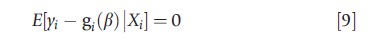
where g_i(β)=[g(x_i1,β),…, g(x_iT,β)]` and X<sub>i</sub> =[x<sub>i1</sub>,…,x<sub>iT</sub>]`.

Although the foregoing analysis is for additive errors, there are multiplicative versions of moment conditions that will lead to different estimators. Because of the greater potential for having omitted factors in panel models of observational data, fixed and random-effect panel count models are more flexible and plausible alternatives to the PA model.

Random Effects Models

A REs model treats the individual-specific effect a_i as an unobserved random variable, uncorrelated with the regressors x_i1,…,x_iTi , with specified mixing distribution g(a_i|y), analogous to the cross-section case. Then a_i is eliminated by averaging over its distribution – an operation which is mathematically equivalent to integrating out ai from the conditional distribution f(y_it|x_it,a_i,β,y). The resulting unconditional density for the ith observation is f (y_it,…,y_iTi|x_i1,…,β,y,η) may have an analytical closed form for some combinations of {f(·), g(·)}, but in general it is handled numerically. Randomness restricted only to the intercept is easier to handle numerically than when it applies to both intercept and slope parameters, which means that the RE is not separable, as in an FMM.

As in the cross-section case, the NB panel model can be derived under two assumptions: first, y_ij has Poisson distribution conditional on μ_i and second, mi are independent, identically distributed (i.i.d.)-y distributed with mean m and variance am2. Then, unconditionally y_ij~NB(μ_i.μ_i +aμ²_i). Although this model is easy to estimate using standard software packages, it has the obvious limitation that it requires a strong distributional assumption for the random intercept and it is only useful in the special case when the regressors in the mean function μ_i=exp(x`_iβ) are time invariant.

A potential limitation of the foregoing RE panel models is that they may not generate sufficient flexibility in the specification of the conditional mean function. Such flexibility can be obtained using a finite mixture or latent class specification of RE.

Fixed Effects Models

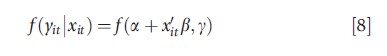
Given the conditional mean specification

a FEs model treats a_i as an unobserved random variable that may be correlated with the regressors x_it. Such dependence may be present if one or more regressors are endogenous. In this sense the FE model deals with a limited form of endogeneity. It is known that ML or moment-based estimation of both the PA Poisson model and the RE Poisson model will not identify β if the FE specification is correct. The main difficulty in handling the otherwise more attractive FE model is that, in general in nonlinear panel models, the nuisance parameters a_i cannot be easily eliminated from the model, which is the incidental parameters problem.

However, under the assumption of strict exogeneity of x_it, the basic result that there is no incidental parameter problem for the Poisson panel regression is now established and well understood. The conditional likelihood principle can be used to eliminate a and to condense the log-likelihood in terms of β only.

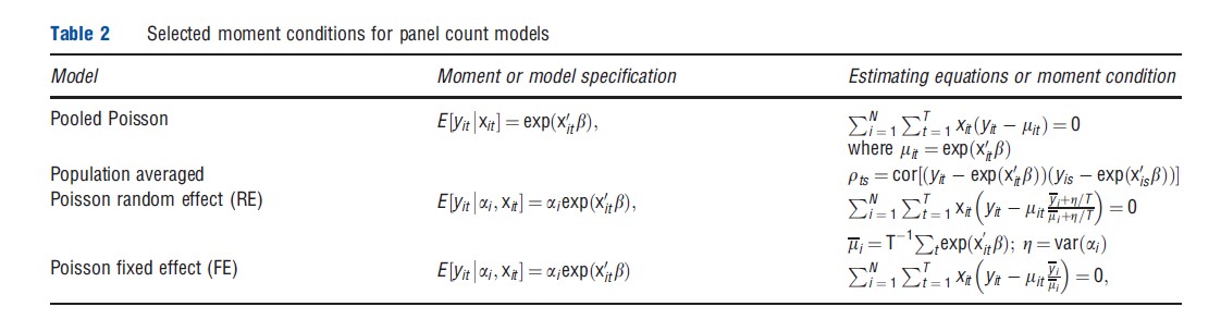
Table 2 below displays the first-order condition for FE PMLE of b, which can be compared with the pooled Poisson first-order condition to see how the FEs change the estimator. The difference is that μ_it in the pooled model is replaced by μ_ity_i/μ_i in the FE PMLE, where μ_i=T^-1∑_texp(x_it`β) and y_i=T^-1∑_ty_it are time averages The multiplicative factor y_i/μ_i is simply the ML estimator of a_I; this means that the first-order condition is based on the likelihood concentrated with respect to a_i.

The result about the incidental parameter problem for the PMLE model does not extend to the FEs NB1 model (whose variance function is quadratic in the conditional mean) if the FEs parameters enter multiplicatively through the conditional mean specification. This fact is confusing for many practitioners who observe the availability of the FEs NB option in computer packages.

Moment Function Estimation

Modern literature considers and sometimes favors the use of moment-based estimators that may be potentially more robust than the MLE. The starting point here is a moment condition model which mimics the differencing transformations used to eliminate nuisance parameters in linear models, that is, moment condition models are based on quasi-differencing transformations that eliminate FEs. This step is then followed by application of one of the several available variants of the GMM estimation, such as two-step GMM or continuously updated GMM.

Two alternative formulations are

where, in the first case E(u_it) =1, the x_it are predetermined with respect to u_it, and u_it are serially uncorrelated and independent of a_i. A quasi-differencing transformation eliminates the FEs and generates moment conditions whose form depend on whether one starts with eqn [11] or eqn [12]. Several variants are shown in Table 2 and they can be used in GMM estimation. Certainly, these moment conditions only provide a starting point and important issues remain about the performance of alternative variants or the best variants to use. In essence these specifications lead to GMM estimation which differ in terms of the weights attached to the moment conditions.

Conditionally Correlated Random Effects

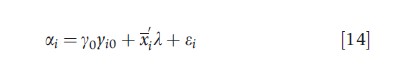
Given the difficulty of eliminating FEs for any flexible functional form, an extension of the RE model offers an attractive alternative. The standard RE panel model assumes that a_i and x_it are uncorrelated. Instead, suppose that they are conditionally correlated. This idea, originally developed in the context of a linear panel model, can be interpreted as a compromise between fixed and random effects, that is, if the correlation between a_i and the regressors can be controlled by adding some suitable regressors, then the remaining unobserved heterogeneity can be treated as random and uncorrelated with the regressors. Although in principle a subset of regressors may be introduced, in practice it is more parsimonious to introduce time-averaged values of time-varying regressors. This is the conditionally correlated random effects (CCRE) model. This formulation allows for correlation by assuming a relationship of the form

where x denotes the time average of the time-varying exogenous variables and ε_i may be interpreted as unobserved heterogeneity uncorrelated with the regressors. Substituting this into the above formulation essentially introduces no additional problems. To use the standard RE framework, however, it is needed to make an assumption about the distribution of et and this will usually lead to an integral that would need evaluating. Estimation and inference in the pooled Poisson or NLS model can proceed as before. This formulation can also be used when dynamics are present in the model.

Dynamic Panels

As for linear models, inclusion of lagged values is appropriate in some empirical models. An example is the use of past research and development expenditure when modeling the number of patents. When lagged exogenous variables are used, no new modeling issues arise from their presence. When lagged dependent variables are introduced, for example, y_it=exp(yy_it-1+x_it`β+a_i), additional complications arise. First, in short panels, initial condition y_i0 will have a persistent influence. Second, the presence of zero outcomes or large lagged outcomes can induce instability. The literature offers a number of solutions whose suitability should be determined on a case by case basis. However, a relatively simple and appealing solution of the initial condition problem is to embed the dynamics in a CCRE model by assuming that where the individual-specific effect absorbs the initial condition. Finally, the i.i.d. component ε_i can be dealt with using the RE framework for the panel data. Estimation of such a model may entail numerical integration to deal with the i.i.d. error and/or the initial condition.

References:

1. Cameron, A. C. and Trivedi, P. K. (1986). Econometric models based on count data: Comparisons and applications of some estimators. Journal of Applied Econometrics 1, 29–53.
2. Cameron, A. C. and Trivedi, P. K. (2009). Microeconometrics using stata revised edition. College Station, TX: Stata Press.
3. Cameron, A. C. and Trivedi, P. K. (2013). Regression analysis of count data, 2nd edn. New York: Cambridge University Press.
4. Deb, P. and Trivedi, P. K. (2002). The structure of demand for medical care: Latent class versus two-part models. Journal of Health Economics 21, 601–625.
5. Gourieroux, C., Monfort, A. and Trognon, A. (1984). Pseudo maximum likelihood methods: Applications to Poisson models. Econometrica 52, 701–720.
6. Hausman, J. A., Hall, B. H. and Griliches, Z. (1984). Econometric models for count data with an application to the patents – R and D relationship. Econometrica 52, 909–938.
7. Koop, G., Poirier, D. and Tobias, J. (2008). Bayesian econometric methods. New York: Cambridge University Press.
8. Machado, J. and Santos Silva, J. (2005). Quantiles for counts. Journal of American Statistical Association 100, 1226–1237.
9. Mullahy, J. (1986). Specification and testing of some modified count data models. Journal of Econometrics 33, 341–365.
10. Trivedi, P. K. and Munkin, M. (2010). Recent developments in cross-section and panel count models. In Ullah, A. and Giles, D. (eds.) Handbook of empirical economics and finance, pp. 87–131. London: Francis and Taylor.
11. Windmeijer, F. (2008). GMM for panel count data models. Advanced studies in theoretical and applied econometrics 46, 603–624.
12. Winkelmann, R. (2003). Econometric analysis of count data. Berlin: Springer-Verlag.
13. Wooldridge, J. M. (2005). Simple solutions to the initial conditions problem in dynamic, nonlinear panel data models with unobserved heterogeneity. Journal of Applied Econometrics 20, 39–54.