Missing Data Weighting and Imputation

Introduction and Goals

Missing Data And Their Consequences

Missing data are common occurrences in health economics and health outcomes research. The patterns of missing data can take many forms. Item missingness occurs when values are missing for selected variables (items) for a subset of subjects or cases; often the subset of cases missing one variable may not be identical to those missing another variable, thus compounding the problem. In contrast, case (record) missingness occurs when subjects selected for a study might have only minimal available data because they might be unreachable or even decline to participate. In panel (longitudinal) data, subjects might not be missing, but records for some waves might be. Dropouts are common, just as intermittent missing data arising when a subject misses a wave but participates in subsequent waves.

Missing data, even if relatively modest in scope, present a major problem when their frequency and structure call into question the validity of and conclusions from statistical analyses of a research study. The two main statistical issues are increased variability and bias. As a general rule, the loss of information resulting from the missingness increases the variability of statistical estimates, sometimes dramatically so, resulting in decreased power for hypothesis tests and wider confidence intervals. A more serious problem is bias, that is, systematic error that may result when the missing data occur disproportionately across subjects or records. Selection bias, which typically occurs when the individuals in the sample are not representative of the target population, may also be induced by nonresponse. The missing data may therefore result in reduced generalizability of study results, and may complicate statistical analyses through the need to mitigate bias.

Statistical Approaches To Missing Data: Overview

Analytic strategies for handling missing data have a long history and fall into several broad categories. The authors mention a few approaches here, and then in Sections ‘Weighting’ and ‘Multiple Imputation’ elaborate two of the most useful and popular ones for missing data.

Historically, methods were focussed on simple imputation of missing values with the aim of conducting analyses using statistical tools that required complete data. Simple imputation techniques such as unconditional mean imputation – replacing missing values with the sample mean of nonmissing values – or carrying the preceding nonmissing observation forward in a panel study were standard approaches. Conditional mean imputation improved slightly on these approaches as it replaces missing values with their sample mean on the basis of a regression model or a sample subset of the full data that is closer in some sense to the record with the missing data. In some settings, this method will yield reasonably unbiased estimators, but will often understate statistical uncertainty and inflate test statistics. Carrying the preceding nonmissing observation forward in panel studies is not recommended.

The most common strategy for handling missing data, complete-record analysis, is to simply delete the records for which data are missing, and base the analysis only on the observations without missing data. In univariate response problems, complete-record analysis ignores data on all subjects for whom some data are missing for a given analysis. In panel data, a subject may contribute data, but records for waves with missing data are ignored. This is referred to as available subject/complete-record analysis. (A subject without any missing items or waves is called a complete subject.) There is really no statistical principle guiding these decisions; rather it is mostly a matter of simplicity and convenience for software developers and analysts. Besides possible problems of bias and inefficiency, complete-record analyses suffer from the problem of different sets of records being included in different model fits, depending on the variables included in the model.

Modern methods for handling missing data frame the problem in terms of a pair of auxiliary statistical models: A model for the distribution of the missing values, and a model for the probability that a given value is missing, sometimes called the missingness mechanism. Sensitivity of inferences to these model specifications, and manipulation of them in order to obtain inferences, has been the topic of a vast missing data literature.

A minimal goal of any method is that it yields valid statistical inferences. For a method to be valid, it should produce consistent (i.e., unbiased in large samples) estimators of the parameters of interest, which are accompanied by consistent estimators of uncertainty (e.g., appropriate standard errors), thereby yielding correct test statistics and confidence intervals. Statistical efficiency (i.e., optimal use of the available data under acceptable modeling assumptions) is another important statistical desideratum.

With these three criteria in mind, one large body of approaches involves correcting bias and generating valid standard errors in complete-record analysis. Whereas other techniques are available, the most common of such approaches is the statistical weighting of complete records. In this approach, efficiency is more of a secondary concern. A key feature of weighting approaches is that a model for the distribution of the missing quantities is not needed. A model for the missingness mechanism is, however, needed in order to generate the weights.

At the opposite end of the spectrum from weighting lies full maximum likelihood estimation, which jointly estimates the model of interest and the model for the missing quantities. Maximum likelihood places the two issues of bias and efficiency on equal footing. If the models are close to correctly specified, then bias will be eliminated, and the solution will be statistically efficient. However, bias and/or inefficiency can arise under misspecification. This approach is also limited because often the analysis of interest (i.e., the analysis one would do in case of no missing data) is not based on maximum likelihood.

For purposes of approximating maximum likelihood estimation, more advanced and flexible imputation techniques have been proposed. The simplest of these is conditional imputation, in which a probability model is specified and estimated for the missing quantities as a function of other nonmissing variables. A random draw from that model is then used to impute each missing value. This method improves on conditional mean imputation because it captures the variability in the data that would have been observed if they had not been missing. For small amounts of missing data, this method can work well. It is convenient and quick, not much more difficult than conditional mean imputation, and data preserving too. Its disadvantage is that the resulting measures of statistical uncertainty will be anticonservative because the approach does not account for the additional variability arising from having estimated the imputation model. Multiple imputation (MI) resolves this issue.

Goals For The Article

It is beyond the scope of this article to cover all missing data methods or to cover any one method in detail. Rather, the authors’ main goal is to introduce key concepts and to provide some guidelines to help the analyst narrow down problems so that he/she may further research specific solutions. With this in mind, in the remaining sections, the authors will focus on the following three objectives. First, a discussion of missing data identifying assumptions, especially missing at random (MAR) and its variants, will be provided. Second, some leading case patterns of missing data with probably valid approaches in those settings will be discussed. Third, two model-driven approaches that are commonly used now, namely, complete-record analysis with weighting, and MI will be described in some more detail. Conditional single imputation, which is described above, is a special case of MI, so that approach will be implicitly covered as well. To focus the discussion, regression problems for univariate or for longitudinal (panel) data will be emphasized. Wherever needed, the settings of missing predictors and missing responses (e.g., attrition) will be differentiated. Also, the authors will emphasize statistical methods for MAR data. Such methods are generally easier to carry out than those for nonignorable missingness, and are more broadly applicable than those analyses that require the relatively severe assumption of missing completely at random (MCAR).

This article focuses on data that are missing by happenstance. There are many situations wherein data are missing by design, either at the item level or at the record or the unit level. Important examples include two-phase sampling designs, case-cohort designs, and outcome-dependent sampling designs for panel data. Some References: for these designs are given under ‘References:’.

Foundational Issues

Preliminaries And Notation

To fix ideas, suppose that the analysis of interest involves the conditional distribution of response Y given predictors X, denoted as [Y|X]. Response Y may be univariate or, in the case of panel data or multivariate data, a vector. Predictors X are almost always row-vector valued or of higher dimension. For example, in panel data, X might be a matrix with number of rows equal to the length of Y. For clarity of exposition, an independent individual or sampling cluster is referred to as a sampling unit, and observations within that unit are considered as records. Units are considered to be stochastically independent, whereas observations within a unit may be correlated. For example, in a panel study, each participant would be a unit, and repeated waves of measurement would generate a separate record each. In a study of twins, the pair would constitute a unit, whereas each of the twins would yield his/her own record.

It is assumed that without missing data, the target of inference would be restricted to [Y|X]; the marginal distribution [X] would be ignored. Therefore, in structural equations models wherein predictors are latent and are measured imperfectly by a set of manifest indicators, those indicators become part of Y because the measurement model is part of the analysis that takes place in the absence of missing data. Where no further specificity is needed, and recognizing that it is difficult to create a notation that is broadly applicable, Y_o and X_o will denote components of Y and X that are always observed, while those components that are potentially missing (i.e., missing for some individuals) will be denoted by Yu and X_u.

In any analysis, it is important to take account of the pattern of missing data. Item nonresponse arises when the missing quantities Y_u or X_u constitute a set of component variables available in Y and/or X. Missing items may be similar or may vary considerably across units. For example, it may be that due to the sensitive nature of the data, many individuals are missing reports of household income. Alternatively, in a questionnaire with many items, some respondents will skip a few items or sets of items here and there, with no consistent pattern from one respondent to another. Unit nonresponse leads to record missingness, a situation where all of Y is missing, as is most of X. Depending on the sampling frame, some minimal part of X might be available. For example, for a nonresponding household in a sample survey, the investigator would still know the address and some neighborhood characteristics according to census information.

Panel data yield special types of record missingness. Most commonly, some participants drop out of a study, leading to attrition that results in monotone missingness patterns. Alternatively, some participants may not come for a given visit or respond at a given wave, but then respond in later waves, leading to wave nonresponse and intermittent missingness patterns.

For purposes of both formal theory and computational development, it is useful to introduce a variable R encoding the missingness pattern for any given unit. The specific form of R will depend on the nature of the missingness. For example, if the only thing ever missing is a single predictor X_u, then R will be a binary indicator equal to 1 if X_u is observed, and to 0 if X_u is missing. Alternatively, in a panel study with intermittent missingness, R may be a vector of indicators with elements of 1 for observed and 0 for missing waves. R may take other forms that are necessary to fully codify the range of missingness patterns.

Some missing data analyses include auxiliary data Z. These additional variables are observed on all units that are associated with, and hence provide information on, the missing data. Auxiliary data can be quite informative in missing data problems. For example, if a key predictor is clinic-measured body mass index and it is missing on some participants, a reasonable pair of auxiliary variables can be self-reported height and weight. It is assumed that auxiliary variables are not part of the target of inference, i.e., the analyst would ignore Z in studying [Y|X] if there are no missing data. For auxiliary data to be of use, it must be predictive of the missing data Y_u or X_u.

A Taxonomy Of Missing Data Assumptions

Rubin (1976) has proposed a taxonomy of missing data assumptions, which has proven to be enormously successful; almost all modern missing data methods refer to it for formal identifying assumptions. Although his taxonomy is rooted in formal likelihood theory, the main ideas are sketched here, downplaying technical details.

Missing data assumptions are framed in terms of the missing data mechanism. This term does not describe the actual machinery or physical processes that lead to data being missing, but rather the stochastic dependencies of those processes on other variables at play in the analysis. Specifically, missingness mechanism refers to the probability distribution of missingness being conditional on (Y, X), viz. [R|Y, X]. Of course, understanding the physical processes may help the investigator in determining what is reasonable to assume where dependencies in the missing data pattern are concerned. In general, acknowledging and accounting for this probabilistic selection mechanism is central to understanding, developing, and applying modern missing data methods.

Data are considered to be MCAR when the probability of missing data is independent of both missing and observed variables. That is, R is independent of either (Y, X) or, when auxiliary data are available (Y, X, Z). Intuitively, under MCAR, complete records arise as if by a random sample from the population, because whether they are complete or not is unrelated to their realized (observed or unobserved) values. In univariate problems, complete-record analysis is a valid, albeit statistically inefficient, approach under MCAR. In panel data, under MCAR, either available subject/complete record or complete subject analysis will lead to valid but inefficient inferences.

The most common missing data assumption is MAR. Under MAR, R is independent of (Y_u, X_u) given (Y_o, X_o) or, in the case of auxiliary data, given (Yo, X_o, Z). Under MAR, the distribution of unobserved data (Y_u, X_u) when R=0 could deviate from that when R=1, but not when controlling or stratifying on (Y_o, X_o, Z). That is, for a fixed value of (Y_o, X_o, Z), the values (Y_u, X_u) for R=1 (or R=0) are a random draw from their conditional distribution [Y_u, X_u|Yo, X_o, Z]. MAR is a weaker assumption than MCAR (MCAR is a special case of MAR), but still yields identifiable models. Intuitively, the implication is that it is possible to model this conditional distribution, thus enabling generation of imputed values for (Y_u, X_u) for those subjects where they are missing. This intuition for model identifiability holds even if imputation is not formally pursued as an analysis strategy. Note that auxiliary data Z can be an important factor in meeting the MAR assumption; intuitively if Z is predictive of Y_u or X_u, it can lead to valid imputations of the missing values, imputations that would not have been available in the absence of Z.

It is useful to consider two special cases of MAR. In the first, missingness of Y_u or X_u only depends on the other covariates X_o, but not on Y_o or any auxiliary data. Because interest lies in the conditional distribution [Y|X], it is possible to treat this covariate-dependent missingness essentially as MCAR. Alternatively, if missingness depends on Y_o, the authors have a true MAR situation and must account for this more carefully in subsequent analyses. Two key examples of this situation are as follows. In the first, a covariate X_u is sometimes missing, and whether or not it is missing depends on the response Y. For example, X_u may be a clinical laboratory test and the ordering of the test may be related to response Y. The second arises in panel data with attrition, where Y_o represents the responses before dropout, and Y_u represents the responses realized but not observed after dropout. This situation is termed sequential MAR if the potential missingness of the responses Y_u (after dropout) depends only on the covariates X and the components Y_o of Y being observed before dropout.

When data are not MAR, they are missing not at random (MNAR) or informative. In this case, the fact R that X_u (or Y_u) is missing is associated with its value, even after controlling for always-observed data (Y_o, X_o, Z). When missingness is nonignorable, statistical analyses can be considerably complicated because they require a model for the missingness process, and this model is based on untestable assumptions regarding the relationship of Y_u or X_u to R. As such, sensitivity analyses are often conducted to assess how inferences change over a range of parameter values for the nonignorable missingness process.

MNAR data are often termed nonignorable. The implication is that under MAR, the missingness is ‘ignorable’ in some sense. This is a potentially misleading statement. MAR allows the model to be identified, but the analyst cannot ignore the problem, or does so at his own peril. Indeed, whereas inferences can be safely based on the likelihood for the complete data, MAR missingness is only truly ignorable if what is missing is part of Y when there are no auxiliary data, and also if full likelihood analyses are pursued. That is, inferences based on likelihood [Y_o|X] instead of on likelihood [Y|X] are valid. If, however, it is a component of X that is missing, then a probability model for X_u is required, something that would not have been part of an analysis with no missing data. If nonlikelihood or conditional likelihood methods are being used, a model for the missing data mechanism is required.

Approaches: When To Use What?

Before approaching any analysis, an assessment of missing data should be undertaken. One should quantify how much each variable is missing, and also document patterns of missingness. Are there a few variables missing often, or many variables wherein each is missing very occasionally? What is the relationship among the missingness of different variables? Is it the response of one or more predictors that is missing? It is then important to assess reasons for missingness during the study as this would lead to realistic assumptions regarding the mechanisms of missingness that will aid in the choice of statistical analysis.

Harrell (2001) provides rough guidelines for handling missing predictor variables X_u in univariate regression models. For 5% missingness or less, unconditional mean imputation of X_u will generally work fine. If 15% or less of observations are missing X_u, he recommends imputing it with conditional mean imputation without the response Y in the imputation model. As the missingness approaches 15%, standard errors may begin to be underestimated. If the missingness R is associated with Y (something that can be examined with the data), this approach will also begin to break down. For analyses where more than 15% of observations have at least one missing predictor and/or where missingness is strongly associated with the response, incorrect modeling assumptions could begin to introduce bias, and standard errors need to account for missing data. Weighting or MI (Section ‘Multiple Imputation’) is recommended.

For the missing responses Y_u in univariate models, if MAR can be assumed without auxiliary data Z, then completerecord analysis will yield valid and efficient inferences. If there are auxiliary data Z, one should examine whether they predict Y_u and/or missingness of Y_u (i.e., R). If Z is strongly predictive of Yu but not related to missingness R, then imputation will increase statistical efficiency. If Z is related to R but not very strongly to Y_u, then weighting as a function of (Z, X) will help to avoid bias. If Z is related to both R and Y_u, then imputation is recommended to avoid bias and maximize statistical efficiency. In any case, for 5% missingness or less, completerecord analysis should work fine.

For panel data with MAR responses Y_u, for example, due to attrition, if the missingness only depends on X, but not on observed responses Y_o, available subject/complete records analysis using either maximum likelihood or semiparametric moment-based methods will yield valid and efficient inferences. If the missingness of Yu also depends on Y_o, the best approach depends on the type of analysis being pursued. If the model is a full probability model with no auxiliary data Z, which otherwise would be fitted with maximum likelihood in the absence of missing data, then one should pursue the same approach on available subjects/complete records. In settings where a moment-based analysis is desired or where auxiliary data Z are available, then other approaches are required. Imputation is a possibility but it can be difficult to implement with both variably spaced observations and dropout at different waves in the study. Weighting is an alternative approach that relies on a model for the missingness or the dropout probability (see Section ‘Weighting’). As this is a binary data model, modeling strategies for the missingness are straightforward to implement with sufficient flexibility. Covariate missingness in panel data is a more complex situation and beyond the present scope.

Weighting

Univariate Data

The general practice of weighting observed data to account for missing data comes from weighting for nonresponse in sample surveys to correct for bias. Briefly, when nonresponders differ from responders according to their distribution of measured characteristics, the responders’ data are weighted so that analysis restricting to the complete data sample would resemble the analysis of the combined data of responders and nonresponders in the case where it had been observed. Use of weights assumes knowledge of some variables such as demographic characteristics, to be available on the nonresponders so that they can be placed in groups or bins with responders. The bin-specific inverse probability of being a responder is then calculated and used as the weight for observations in that bin. The same principle can be applied in a prospective study where the outcome Y at the end of the follow-up period is missing for some subjects. The general idea is to weight records inversely to their probability of being observed such that observed data with a low likelihood of being observed receive relatively high weight. When incorporating continuous as well as categorical baseline variables, instead of bins, a logistic regression model can be used to estimate the probability of being observed at follow-up for each study participant. The resulting inverse probability is then the weight used in the complete-data analysis for the outcome. The same general method of constructing weights applies to missing covariates in regression settings. When more than one covariate is missing or when missing data patterns for repeated measures are nonmonotone, implementation of weighting strategies becomes less straightforward. The next section considers the special problem of weighting for missing data due to subject dropout in panel data.

Weighted Estimating Equations For Panel Data With Dropouts

A common problem in panel studies is subjects dropping out before study completion. Whereas subject-specific random effects models estimated with maximum likelihood are a popular approach to the analysis of longitudinal data, another approach is population-averaged modeling of marginal means. Such semiparametric estimation of marginal mean regression models is especially attractive for discrete outcomes because specification of their full joint distribution is not needed. In particular, a semiparametric estimation approach using record-specific weights derived from a model for dropout addresses potential bias due to sequential MAR dropout.

To define the problem, assume that there is a set of T planned measurement times being common to all individuals, and that interest lies in the mean μ_t of response Y_t across times t=1,…,T. However, some subjects drop out of the study before T, thereby creating a monotone pattern of missingness. Letting t’ be the final observation time before dropout (for a given subject), Y_o = (Y₁,…,Y_t’), Y_u = (Y_{t’ +1},…,Y_T), and Y = (Y_o, Y_u) is obtained. To indicate missing data, R=(R₁,…,R_T) is also obtained, where R_t=1 for t≤t’ and 0 otherwise. Next let X_t be the covariate vector which is used to predict μ_t, so that μ_t is a function of X`t_β. Assume that all X_t’s are known, as is the case, if all covariates are baseline characteristics (time-independent) or deterministic functions of known quantities such as the planned measurement times, or are external to the measurement process.

Generalized estimating equations (GEEs) provide a common approach to marginal mean regression modeling for panel data while accounting for correlation among an individual’s repeated responses. With dropout, GEE estimates β by solving the equations

where the sum is over all subjects in the panel. Here, μ₀=(μ₁,…,μ_t`), and V_o^-1 is the inverse of the working covariance matrix of Y_o (i.e., the observed part of Y). D_o=δμ_o/δβ and is a generalization of X_t in the normal equations of a linear regression model. GEE yields a consistent estimate of β even if the covariance structure is misspecified, provided the missing data are MCAR or when missingness depends only on covariates X_t. However, under MAR, a GEE analysis generally gives biased estimates.

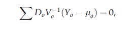
In contrast, weighted GEE (WGEE) is valid under MAR even if the covariance structure is misspecified, provided the model for the probability of dropout is correctly specified. WGEE modifies GEE by solving instead the equations

where μ, V^-1, and D now correspond to the full data vector Y, both observed and unobserved components, and W is a diagonal weight matrix with components R_tw_t, t=1,…,T. Note that, because W is diagonal, it multiplies, or weights, each element (Y_t-μ_t) of (Y-μ) by R_tw_t. As in univariate data, w_t is equal to the inverse probability of the tth record being observed, and R_t selects the observed components of Y. In the case of a working independence covariance assumption, V is diagonal, and WGEE reduces to GEE, where W_o is diagonal with elements w₁,…,w_t` . Compared to WGEE with a nondiagonal working correlation matrix, independence WGEE is rather straightforward to implement as it utilizes the same data structure as the independent GEE, with little efficiency loss when the number of subjects is large.

The benefits of WGEE relative to GEE are twofold. First, just as with the univariate analysis already described, the inverse probability weights in W serve to correct the bias due to nonresponse at the record level. Second, through the working correlation structure posited in V, multiplying by V_-1 serves to implicitly impute components of Y_u via the observed data in Y_o. There are three main steps in implementing WGEE:

Step 1: Determine observation-specific weights w_t, t=1,…,T, through a model for the missingness.

Step 2: Apply the weights to W in the WGEE equations and solve to estimate the β parameters in the marginal mean model for μ_t.

Step 3: Calculate the empirical sandwich-type estimator of the variance–covariance of β with the estimation of weights taken into consideration.

In Step 1, under sequential MAR, let λ_t denote the conditional probability that Y_t is observed, given Y_t-1 is observed. This probability is typically modeled with logistic regression of R_t on X, prior responses Y₁,…,Y_t-1, and possibly auxiliary data Z. Weight w_t is the inverse of the unconditional probability of being observed at wave t, estimated as the inverse of the cumulative product of conditional probabilities, w_t^-1=λ₁×…×λ_t.

With weights fixed in Step 2, β estimation is similar to that in classical GEE, alternating between regression and covariance parameter estimation. Under correctly specified models for the marginal means and the dropout process, WGEE yields a consistent asymptotically normal estimator of β. In Step 3, a sandwich estimator is generally used. This estimator is biased for the true variance of β, because it treats the weights w_t as fixed even though they are estimated. In contrast to sampling theory, where fixed weights are used, semiparametric theory provides that this version of the weighted sandwich estimator tends to overestimate the true variance so that options for specifying fixed weights in widely available software for GEE tend to provide conservative estimates of the standard errors for β.

In summary, the WGEE procedure corrects for bias when the GEE assumption of MCAR is in doubt. A few caveats are in order. As in GEE, choice of the working correlation structure in WGEE may affect efficiency. A particular concern with the WGEE method is that misspecification of the missingness model may cause bias in β, which can even exceed that of GEE. Accurate choice of the working correlation can mitigate this problem. As with sample survey weights, caution should be used in applying very large weights. Finally, more complex extensions of this procedure are needed to mitigate efficiency loss.

Multiple Imputation

Overview

For relatively small amounts of missing data, single imputation is an approach that has many advantages. It is valid under MAR and can easily incorporate auxiliary data in the imputation model. It fully exploits the available data. Because data can be imputed before analyses, a single set of imputations can support multipleanalyses. Indeed, the imputation can even be done by a different data analyst other than the final data analyst. Single imputation replaces missing values with those drawn from a fitted distribution, obtained via the nonmissing values. Being drawn from a distribution, the missing values retain the same variability that would be seen if the data had not been missing.

The main disadvantage to single imputation is that it does not account for the fact that the model for imputing the data is itself estimated from the data and not known a priori. Specifically, once data are imputed, the final analysis produces estimates and standard errors as if the data are complete. MI solves this problem, thereby providing a complete inferential framework for conducting any type of statistical analysis when there are missing data.

MI proceeds via a three-step process. For ease of exposition, the authors sketch that process for the problem of imputing possibly multivariate missing predictors X_u; the process is similar for other missing data patterns, for example, if the missing data are Y_u.

Step 1: Posit a Bayesian model for [X_u|, X_o, Z; ϕ], governed by parameter ϕ. Specify a prior for ϕ and use the data with Bayesian inference to generate a posterior distribution for ϕ.

Step 2: Randomly draw a value ϕ from the posterior distribution of ϕ.

Step 3: For each missing X_u, randomly impute from the distribution [X_u|Y, X_o, Z; ϕ]. Steps 2 and 3 are repeated M times to produce M imputed ‘complete’ data sets. The M data sets can then be analyzed using any valid statistical procedure. Historically, M was set at 5 or 10; with experience, methodologists have learnt that M=20 often provides more reliable statistical performance with insignificant increases in computing costs or analyst’s time.

MI yields several important advantages over other methods for handling missing data. The M imputations can be generated independently of the analysis using whatever variables are available. The analyst neither needs to explicitly account for the exact specification of the imputation model [X_u|Y, X_o, Z; ϕ] nor for the auxiliary variables Z being used in the imputation. Rather, all necessary information to make inferences is contained in the M imputed data sets. In particular, because each imputation is based on a different draw ϕ from the posterior of ϕ, the MIs capture the additional uncertainty due to the estimation of the imputation model. One implication is that the imputations can be generated as part of preliminary data processing, before generating analysis data sets. For example, in a publicly available national survey, the organization performing the survey can generate the imputed data sets and make them available for download with the original nonimputed data. A final advantage is that MI, via modern Bayesian resampling methods, is capable of flexibly handle both monotone and nonmonotone missing data patterns.

Computational Details

It is beyond the scope of this article to cover the statistical theory underlying MI. Nevertheless, it is useful to present the few central formulae prevailing in all MI routines, partly because they emphasize the simplicity and portability of the method across various analysis settings and approaches, and partly because they provide a vehicle for explicating about how MI incorporates the uncertainty due to missing data into the final analysis.

Picking up from Step 3 above, analysis is completed in two additional steps. Assume that interest lies in parameter θ governing [Y|X; θ]. For ease of exposition, the authors assume that θ is unidimensional. The extension to multidimensional θ is straightforward, but involves both vector and matrix arithmetic, and is therefore more challenging to present.

Step 4: For each j from 1,…,M, the jth imputed data set is analyzed as if the data are complete, obtaining estimates θ^(j) with corresponding standard errors √V^(j).

Step 4 is repeated M times. Note that any type of analysis can be pursued to obtain estimates θ^(j) and standard errors V^(j). This could, for example, be a maximum likelihood or a generalized method of moment-based analysis. The key assumption is that the sample size is large enough for the θ^(j) s to be approximately normally distributed. Of practical importance, the repeated analysis in Step 4 can in almost all cases be automated, and several modern statistical packages (e.g., SAS and Stata) have written MI wrappers that can be applied to any standard analysis being available in the package.

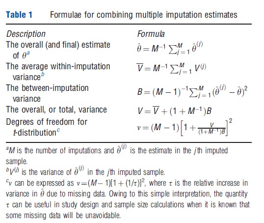
Step 5: Estimates θ^(j) and √V^(j) are combined to yield final estimates θ and √V, using the formulae shown in Table 1. In particular, the overall (and final) estimate of θ is the average of the M estimates. The overall variance V is comprised of two parts, the average within-imputation variance and the (scaled) between-imputation variance. The overall standard error √V can be used in the usual way to construct normal or t-based hypothesis tests and confidence intervals. Owing to the fact that M is usually not large, Rubin (1987) has recommended about using the t-distribution with n degrees of freedom (df) for critical values, where n is given in Table 1. Notably, v goes to ∞ as M becomes large, or, for fixed M, as the amount of missing data become small. Specifically, as the proportion of missing data shrinks, the imputation specific estimates θ^(j) will become closer and closer to one another so that the betweenimputation variance will naturally shrink to zero, causing v to go to ∞.

Multiple Imputation In Practice

To implement MI in practice, the imputer needs to specify a model for [X_u|Y, X_o, Z; ϕ] as well as a prior for ϕ. For continuous components of X_u, the model is often based on linear regression, whereas for categorical, it is often based on logistic regression as well as its extensions for categorical and ordinal data. There is considerable benefit in having this model be fairly flexible, so if the sample size supports it, one should include nonlinear terms for continuous predictors as well as key pairwise interactions between predictors. Vague priors are generally used in an attempt to reflect a state of relative ignorance regarding ϕ.

Monotone missingness patterns are more straightforward to model because the joint distribution of all components of X_u can be modeled via a series of conditional models. In more complex nonmonotone missing data patterns, full conditional resampling methods are often used, wherein one component of X_u is modeled and imputed on the basis of imputed values of all the other missing components of X_u. This process is iterated with new samples of f and all components of X_u in order to generate M imputed data sets.

In modern statistical packages, much of the missing data modeling and imputation is handled in procedures that automatically determine the scale of each component of X_u, specify a default model, determine whether the pattern is monotone or not, specify a prior for f, and ultimately generate the imputed data sets. Default specifications can be overridden, but with modest levels of missingness, the defaults are often perfectly adequate. Those same packages often contain tools for carrying out the postanalysis summaries and inferences as described in Step 5 above. MI for clustered or longitudinal data is less systematically implemented in standard software packages. These situations are more complicated, especially if the data are imbalanced.

Finally, a comment regarding robustness. Certainly, there is a need for model flexibility in order to capture the key relationships of X_u to (Y, X_o). And, with a fairly extensive modeling machinery needed for complex missing data patterns, there are plenty of opportunities for misspecification. Nevertheless, simulation work and empirical evidence have shown that final inferences for θ are often quite robust to specifications of the missing data model. It is believed that the underlying reason for this is that most data are not missing. In most cases, less than 30% of data are missing, often even less. Hence, there is much to be gained by doing imputations even if the imputation model is only correct to first order. The degree to which incorrect models can lead to bias is in some sense bounded by the fact that at most 30% of the data (or whatever percent are missing) are the result of such incorrect model specifications. There is only so much damage that modest model misspecifications can inflict, especially when contrasted with the potential bias in carrying out naive complete-record analyses.

Conclusion And Key Literature

Missing data occurs in many if not most applied data analysis settings and can introduce bias and inefficiency if not handled properly. Quantifying the extent and structure of missing data is key to choosing appropriate methods, and this should be done using the framework of MCAR, MAR, and MNAR missingness. Two popular, widely applicable, and flexible methods are weighting and MI. These are valid under MAR missingness. Not being discussed here, NMAR missingness is especially challenging but can be approached via sensitivity analyses in the model for the missingness mechanism.

Seminal works in this area include Rubin (1976, 1987), Little and Rubin (2002), and Robins et al. (1995). Useful References: are Schafer (1997) and Schafer and Graham (2002). Other References: drill deeper on the topics discussed here or discuss related work.

References:

1. Harrell, F. E. (2001). Regression modeling strategies. New York: Springer.
2. Little, R. J. A. and Rubin, D. B. (2002). Statistical analysis with missing data (2nd edn.). New York: John Wiley.
3. Robins, J. M., Rotnitzky, A. and Zhao, L. P. (1995). Analysis of semiparametric regression models for repeated outcomes in the presence of missing data. Journal of the American Statistical Association 90, 106–121.
4. Rubin, D. B. (1976). Inference and missing data. Biometrika 63, 581–592.
5. Rubin, D. B. (1987). Multiple imputation for nonresponse in surveys. New York: Wiley.
6. Schafer, J. L. (1997). Analysis of incomplete multivariate data. London: Chapman & Hall.
7. Schafer, J. L. and Graham, J. W. (2002). Missing data: Our view of the state of the art. Psychological Methods 7, 147–177.
8. Breslow, N. E. and Cain, K. C. (1998). Logistic regression for two-stage casecontrol data. Biometrika 75, 11–20.
9. Briggs, A., Clark, T., Wolstenholme, J. and Clarke, P. (2003). Missingypresumed at random: Cost-analysis of incomplete data. Health Economics 12, 377–392.
10. Hogan, J. W., Roy, J. and Korkontzelou, C. (2004). Handling drop-out in longitudinal studies. Statistics in Medicine 23, 1455–1497.
11. Horton, N. J. and Lipsitz, S. R. (2001). Multiple imputation in practice: Comparison of software packages for regression models with missing variables. The American Statistician 55, 244–254.
12. Little, R. J. A. (1995). Modeling the drop-out mechanism in repeated measures studies. Journal of the American Statistical Association 90, 1112–1121.
13. Perin, J., Preisser, J. S. and Rathouz, P. J. (2009). Semi-parametric efficient estimation for incomplete longitudinal binary data with application to smoking trends. Journal of the American Statistical Association, Applications and Case Studies 104, 1373–1384.
14. Preisser, J. S., Lohman, K. K. and Rathouz, P. J. (2002). Performance of weighted estimating equations for longitudinal binary data with drop-outs missing at random. Statistics in Medicine 21, 3035–3054.
15. Prentice, R. L. (1986). A case-cohort design for epidemiologic cohort studies and disease prevention trials. Biometrika 73, 1–11.
16. Rathouz, P. J. (2003). Likelihood methods for missing covariate data in highly stratified studies. Journal of the Royal Statistical Society, Series B 65, 711–723.
17. Schildcrout, J. S. and Heagerty, P. J. (2008). On outcome-dependent sampling designs for longitudinal binary response data with time-varying covariates. Biostatistics 9, 735–749.
18. Schildcrout, J. S. and Rathouz, P. J. (2010). Longitudinal studies of binary response data following case-control and stratified case-control sampling: Design and analysis. Biometrics 66, 365–373.