Empirical health economists are likely to encounter questions regarding health and health behaviors that involve dynamics. What does one mean by dynamics? Put simply, a dynamic model of economic behavior captures the element of ‘time.’ In contrast, a static model leaves out time. More specifically, intertemporal dependence is made explicit in dynamic models. This article discusses some of the econometric methods used to estimate dynamic empirical models.
To motivate these methods, the article begins with three examples of individual behaviors studied by health economists that exhibit meaningful relationships across time. Building on these examples, the article presents the econometric methods that have been used by health economists to measure dynamic relationships or behaviors that are connected over time. Much of this work attempts to recover causal effects of variables on outcomes (as opposed to mere statistical correlations) in a dynamic empirical setting. The article concludes with a description of solution and estimation of optimization problems that recover the underlying ‘primitive’ (or structural) parameters that characterize how economists model dynamic decision making.
Examples Of Dynamics In Health And Health-Related Behaviors
As demonstrated in each example in this section, behaviors that are dynamic involve an event, outcome, or action in the past that affects current decisions regarding that behavior or, related, an event, outcome, or action today that impacts future decision making. A distinction needs to be made as to whether the observed event, outcome, or action is endogenous or exogenous. The adjective endogenous implies that the agent (individual or firm) had a role in choosing or influencing the event, outcome, or action; exogenous implies that characteristics of the agent do not affect the event, outcome, or action. Most importantly, endogeneity suggests that unobservable characteristics of the agent likely affect adjacent (in time) behaviors. Another important characteristic of the examples that follow is that the observations of interest are specific to an individual (i) over time (t). We will assume that the econometrician has access to data with repeated observations on the same individuals. We need many observations in the ‘individual’ dimension, but may have only a small number of observations in the ‘time’ dimension.
Example 1: Health Production
It is difficult to think about dynamic models in health economics without thinking of Michael Grossman’s seminal work on health capital and the demand for health (1972). Grossman was the first economist to formally model the optimal health and medical care consumption of individuals. He recognizes, and emphasizes, that health is inherently dynamic. Indeed, time is such an integral part of health-related decision making that Grossman framed it as an optimization problem being solved over a lifetime.
In this example, the evolution of an individual’s health is a dynamic process. Grossman describes our health as a stock, or a capital good. One might compare it to the concept of human capital, or the stock of education that an individual acquires over her lifetime. In fact, similar to education or any capital good (e.g., computer equipment) that a firm uses in production, the stock of health requires maintenance, and depreciates, over time. And, like other capital goods, health can be characterized by its stock and its flow. The stock is an instantaneous measure of current health. The flow is the services or benefits that are generated from a stock of health.
But health cannot be purchased. An individual cannot go to the store to buy more health when her health stock falls below a particular level. Rather, an individual produces health – with the operative words being ‘individual’ and ‘produce.’ The first word signifies that each individual is responsible for their own health stock. This responsibility does not imply that accidents can always be avoided. It is quite true that unfortunate events that reduce our health stock happen, and happen with no fault of our own. Yet, our own behaviors can and do influence our health stock.
That influence is exactly where the second word ‘produce’ comes in. An individual chooses inputs to sustain or augment a health stock. She may also choose inputs that reduce or weaken her health stock. An obvious example of a positive input (i.e., one in which the marginal product is positive) is medical care. If one’s health deteriorates, she may consume medical care to repair it. Other examples, of both positive and negative inputs, include food, cigarette, and alcohol consumption. In addition to market goods that affect health, nonmarket goods may impact health. For example, exercise, sleep, and stress are health inputs.
Given this understanding of health capital economists model it as a dynamic productive process with depreciation. That is, let Hit define an individual’s health stock at time t. Let Iit denote a selected amount of health input at time t. Then, according to the description of the evolution of the health stock, a simple mathematical definition of the dynamic process might be
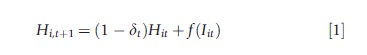
where δt measures the depreciation rate of health capital in each period t to t + 1 and f(·) is a function that converts the period t health input into health next period. Given this definition or model, it should be immediately obvious that the health production process involves time. Health in one period evolves into health in the subsequent period with the help of chosen behavioral inputs during the transition period. Unfortunately, social scientists do not observe an individual’s rate of health depreciation nor do they know with certainty the effectiveness of any one health input for a particular individual. Yet, these are exactly the empirical questions health economists seek to answer when studying health and health behaviors.
Example 2: Addictive Good Consumption
Cigarette consumption was described in Example 1 as a (negative) health input. To measure the effect of cigarette consumption on health outcomes, an econometrician must first understand decisions to smoke. (Smoking is an example of an action that is endogenous. Unobservable individual characteristics that affect smoking might also affect the health outcome of interest, which will bias estimates of the smoking effect.) A simple approach to modeling demand for any good is to consider the demand to be static. That is, today’s demand for a good depends only on measures of specific variables today: an individual’s income today, her current age, the price of the good today, and even the prices of goods that are substitutes for or complements to the good being considered, etc. However, health economists place cigarettes in a different class of goods, namely addictive goods (Chaloupka and Warner, 2000). Other examples of addictive goods might be alcohol, fast food, illicit drugs, etc.
What characterizes an addictive good? The basic premise is that past consumption of the good alters the enjoyment an individual receives from current consumption. That is, the demand for the good today depends not only on measures of specific variables today, but also on measures of specific variables in the past. Herein lies the role of time, or dynamics.
Economists have labeled three ways that past consumption of an addictive good might alter the enjoyment of the good today. The first characteristic of an addictive good is tolerance: The amount of the good consumed in the past directly affects ‘happiness’ today or, in the economist’s terminology, contemporaneous ‘utility.’ Using fast food consumption as an example of a negative addiction, someone who has consumed a lot of greasy French fries in the past is unhappier (all else equal) than someone who has not developed this addiction. However, a beneficial addiction might be to exercise. Tolerance suggests that someone who has engaged in exercise routinely in the past may experience greater happiness today, all else equal.
The second characteristic of an addictive good is withdrawal: Consumption of the good provides positive utility. Put differently, an individual foregoes this utility if they choose not to smoke. Thus, a smoker, who anticipates the reduction in utility today associated with their past use, can look forward to the boost in utility they receive from continuing to smoke today. If they quit, their utility is lower.
The third characteristic is reinforcement: The marginal utility of consumption of the good today is greater when the person has a history of consumption of the good. This characteristic suggests that consumption of the good in two consecutive time periods is complementary. Adjacent complementarity also implies that reducing consumption of the addictive good (or quitting) is harder the more one has consumed in the recent past.
Each of these characteristics suggests that the demand for an addictive good depends on past behavior related to that good. That is, demand is dynamic. Note, however, that this dependence on past behavior also suggests that behavior today will impact optimal future behavior. That is, an individual deciding whether or not to smoke today (and the amount to smoke) takes into consideration their past smoking behavior, but also understands that their decision today will affect their optimization problem regarding the same behavior tomorrow. Hence, today’s decision, which is based on maximizing lifetime utility from this period forward, depends not only on past behavior, but also on expected optimal behavior in the future conditional on today’s choice.
Health economists theorize that the demand for an addictive good (under particular assumptions about the optimization problem of the individual) is described by the function:
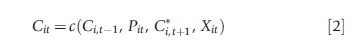
where Cit is current consumption of cigarettes, Ci,t-1 is lagged consumption, and C*i,t+1 is expected future consumption. The contemporaneous price of cigarettes is denoted as Pit and exogenous individual characteristics are denoted as Xit. Given this demand relationship for addictive goods, one can easily see how time plays a role. In particular, consumption of the addictive good in different time periods affects current consumption of the good.
Example 3: Health Insurance Selection
The optimal health insurance decision, or the demand for health insurance by an individual, is another example of a health-related behavior that involves elements of time. More specifically, an individual decides today, without perfect knowledge of her future need for medical care, whether or not to purchase a health insurance plan, which reduces the financial responsibility for medical care consumed in the near future. That is, health insurance is chosen before realization of the health state, and hence, medical care expenses. Put differently, at the point of insurance decision making, medical expenses are uncertain (Arrow, 1963).
A basic, stripped down model of optimal health insurance purchase involves choosing a plan to maximize expected utility. The uncertainty of health, and therefore medical care consumption, requires an individual to forecast – at the time of the insurance decision – the distribution of future medical care expenditure. The decision of an individual to purchase health insurance depends not only on the individual’s expected medical care expenditure (i.e., some average measure), but also on the tails of that distribution. How likely am I to experience a disastrous health event that requires high medical care expenditure?
Suppose the set of health insurance alternatives differ by the level of cost-sharing or reimbursement (which ranges from 0% to 100%) and the premium (i.e., the price of the plan). That is, if an individual chooses a 30/70% plan, the insurance company pays 70% of medical care costs during that insurance year, whereas the individual is responsible for the remaining 30% of total expenses. The premium, or price of insurance, increases with the level of coverage. Assuming utility is a function of wealth, the individual decides on the optimal level of insurance coverage that will maximize her expected utility under uncertain health or medical expense. Specifically, an individual selects insurance as if she were solving the following optimization problem:
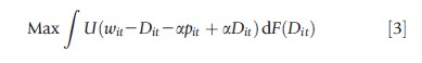
where wit is the individual’s wealth in period t, Dit is the unknown medical care expense at t with known distribution, F(·), and pit is the insurance premium per percentage of payout, a, which measures the level of insurance coverage. In this simplified model, the individual maximizes expected utility by choosing the optimal level of coverage a (which is between 0 and 1 inclusive). Mathematically, the solution involves integrating over the medical care expense distribution, F(·), because costs of medical care are not known with certainty. Therefore, the optimal level of coverage depends on initial wealth, the price of insurance, the individual’s level of risk aversion (captured here by the shape of the utility function U(·)), and finally, the distribution of medical care expenses.
Here, the role of time is a bit more subtle. This example abstracts from the very realistic assumption that previous experience with particular health insurance plans or past medical care utilization may influence the current value of each health insurance alternative; in that case, the role of time mimics previous examples. However, the simple model above highlights a role of time that is different from the previous examples: Optimal decision making requires the individual to forecast future medical care expenses based on current information. Below we discuss how to solve and estimate this dynamic behavior.
The examples presented above relate to individual health behavior. Yet, there are many examples of dynamics on the supply side of health economics. Consider, for example, technology adoption or the decision of a firm to enter or exit the market. How do a firm’s actions today affect the likely actions today or tomorrow of its competitors? The health literature examines these dynamic behaviors in hospital entry and exit, medical equipment adoption, and learning by firms or physicians about drug or procedure effectiveness, just to name a few areas.
Econometric Methods To Capture Dynamics
The first two examples describe the production function for health and the demand function for an addictive good. Equations [1] and [2] depict the relationships between the explained variables (i.e., health and consumption of addictive goods) and the explanatory variables. Economic theory guides the inclusion of particular explanatory, or right-hand side, variables. Then, the economist or econometrician can think about estimating an empirical model that captures the dynamic relationship.
Consider the following steps taken by the econometrician.
Step 1: Specify The Econometric Model
Given a theoretical relationship between variables of interest, the first step is to specify an appropriate econometric model. An econometrician might specify the evolution of health capital, depicted theoretically as the health production function in eqn [1], as follows:
![]()
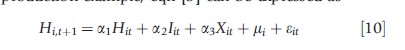
where a1 and a2 are coefficients to be estimated. They reflect the measured effect of the variation in the explanatory variables on variation in the dependent variable. In particular, a1 measures the depreciation of the health stock between periods t and t + 1 and a2 measures the investment in the health stock obtained by consuming an additional unit of the input Iit. The uit term measures the unobserved or unexplained variation in health among individuals. It captures the fact that the relationship between Hi,t + 1 and Hit and Iit is not perfect or, rather, that Hit and Iit do not fully explain Hi,t + 1. Error terms are always added to statistical models that describe behavior of individuals because we are social beings, and our behavior is often not as completely predictable as it might be for many natural or physical behaviors. To avoid introducing too much additional notation, the notation uit is used to capture unobserved heterogeneity, generally, in all the equations that follow. The reader should understand that the amount of error and, hence, the variable that captures that error, depends on the behaviors being explained as well as the power of the observable explanatory variables.
The health production relationship can be made more realistic (and more complicated) by including additional explanatory variables that make sense theoretically. For example, Grossman himself suggests that education influences the marginal product (or effectiveness) of a health input. Let Xit define demographic characteristics of the individual. The econometrician might test the hypothesis that education matters by estimating the following regression:
![]()
It should be noted that the relationship in eqns [4] and [5] holds for all time periods. Thus, the model can be rewritten as
![]()
Turn now to the example of addictive good consumption. The econometrician might specify the equation that depicts the demand function described in eqn [2] as
![]()
where the variables have been previously defined, and the marginal effects of these variables are depicted by parameters, γ, to be estimated.
Step 2: Determine The Measurable Variables To Be Used In Estimation
Having specified the model, the econometrician has to determine whether data exist to estimate the model as it has been specified. For example, how should health stock be measured? What variable exists in a data set that best captures a person’s stock of health? What inputs affect health? Do measures of those inputs exist? Which inputs need to be modeled because they are chosen by the individual? For now, consider only one health input: medical care. Later, the case where multiple inputs may better explain the evolution of health will be considered.
Estimation of the empirical model in the addictive good example requires that the econometrician observe an individual’s consumption and the price of cigarettes over time. In some cases where longitudinal information on individual level consumption has not been available, econometricians have used their knowledge of the dynamic nature of addictive good consumption and the availability of cigarette prices over time to replace past and expected future consumption with the relevant price information at the time of consumption. Hence, eqn [7] becomes
![]()
One can still see that ‘time’ plays an integral role in predicting current consumption. Specifically, prices of cigarettes yesterday, today, and tomorrow may affect cigarette consumption today.
Step 3: Evaluate The Role Of Unobservables Associated With The Dynamics Of The Model
Given a dependent variable (e.g., Hit and Cit in the two previous examples) and a set of observable explanatory variables, one might initially consider the use any one of the statistical estimators described in previous articles. An ordinary least squares (OLS) regression seems like an obvious candidate. However, the dynamic feature of the equations begs the question: Do unobserved individual differences (heterogeneity) that explain the observed lagged outcome (Hi,t -1), action (Ii,t -1), or event (Pi,t-1) in the past also influence the current outcome (Hit) or action (Cit) that is being explored? If so, then the error terms that explain the dependent variable and the right-hand side variable are serially correlated. It may also be the case that these unobservables are heteroskedastic (i.e., the amount of variation in the error differs by observable characteristics), but the focus in this article is on the intertemporal dependence in behaviors, outcomes, and events over time.
First, consider the desire to estimate the effect of an outcome in t-1 (Hi,t-1) on the same outcome in time t (Hit). How might the same unobservable affect both the variables Hit and Hi,t-1? One example must be that of unobserved health. Recall that one of the data questions above was about the measurement of health. It is hard to think of, let alone find in an available data set on individuals, a variable that fully captures one’s health stock. Thus, unobserved measures of health (that are correlated with the observable measure) are captured by the error term, and these unobserved measures of health are likely correlated over time. This endogeneity produces either upward or downward bias in the OLS estimate of the endogenous variable’s effect.
However, an unbiased estimate of depreciation (a1) can be obtained only by using specific econometric techniques to account for the correlation in the unobservables. Other examples of this correlation in measures of health over time are unobserved family health history, unobserved rates of time preferences that capture how forward-looking an individual may be, and unobserved health inputs. One might encounter the same problem when trying to estimate the effect of an action in t -1 (Ci,t-1) on the same action in time t (Cit). Unobservables that affect cigarette consumption today are likely correlated with consumption yesterday.
Now consider a desire to estimate the effect of an action in the past (Ii,t-1) on an outcome today (Hit). Might Ii,t-1 be correlated with Hit through unobservables that affect both? Unobserved health, for example, may be correlated with both medical care decisions and observed health outcomes. That is, lagged observed health Hi,t -1, and thus also lagged unobserved health, may affect both one’s input decisions last period, Ii,t-1, and current realizations of health, Hit. If current unobservables ‘move with’ those past unobservables (i.e., are correlated), then estimated coefficients that measure the effect of these lagged observable variables are contaminated with endogeneity bias (if the econometrician does not address the correlation).
To illustrate more fully, decompose the period t error term (uit) into three components. We want the first component to capture permanent unobserved differences in individuals. We label this permanent heterogeneity mi. These unobserved individual differences do not vary over time, but may affect observed actions or outcomes in each period. Examples of this type of heterogeneity include risk aversion, genetic characteristics, rates of time preferences , or other aspects of the production process or decision-making process that remain fixed over the life cycle. The second component captures time varying unobserved characteristics of individuals that might be correlated with the explanatory and to-be-explained variables. We label this time-varying heterogeneity nit. Examples include unobserved health shocks, stress, or behaviors that may differ each period. The third component, eit, is an identically and independently distributed (iid) unobserved error term that is uncorrelated over time and uncorrelated with each of the explanatory variables of the equation. This last component does not cause any problems econometrically. The first and second must be dealt with appropriately. More formally, the general error term can be decomposed into three components:

As the examples suggest, the unobservables that impact estimation of variable effects may be either permanent (mi) or time varying (nit). There are different econometric techniques that can be used to address these unobservables, depending on the type of variation/correlation.
Step 4: Determine The Appropriate Estimation Method
Economists recognize that dynamic relationships often lead to correlation in variables, or their unobserved determinants, over time. Consider, now, four different methods for addressing the econometric problems associated with unobservables that are correlated over time.
Instrumental Variables
In the case of cigarette consumption (eqn [7]), economists recognize that unobservables that determine smoking behavior in the last period may affect smoking behavior in this period, which will bias the measured effects of lagged smoking on current smoking if not addressed econometrically. One solution is to find another variable that varies across individuals that explains lagged smoking behavior but, conditional on the observed lagged smoking behavior, does not independently impact current smoking behavior. Economic theory suggests that smoking decisions in each period depend on the price of cigarettes in each period. Hence, without measures of lagged smoking behavior, Ci,t-1, one can replace the behavior with its determinants, namely the price of cigarettes in the lagged period, Pi,t-1. Equation [8] above depicts the new equation using this approach.
For this variable to be a valid ‘instrument’ for lagged smoking behavior, the econometrician has to answer several questions. First, does this variable vary over individuals? Individual-level variation in prices is difficult to find, but price series that differ by county or state exist. And prices often vary over time. So, cigarette prices by state of residence and time of consumption usually provides enough variation to identify the effect of prices on individual behavior. Second, might Pi,t-1 be correlated with Ct through unobservables that affect both? If the ‘price’ of cigarettes is measured by any public policy variable such as cigarette taxes or smoking bans in public places, a public finance economist would probably answer this question with a ‘yes’. The political process naturally reflects the preferences of the people, and hence these measures of the costs of smoking are correlated with demand behavior. For the purposes of this article, consider variation in the prices of cigarettes (across states and across time) to be exogenously determined. Thus, there is no need here to worry about unobserved correlation between Pi,t-1 and Cit.
Before stating a third question that must be answered to determine the validity of an instrument, reflect on the specification of eqn [8], which suggests that lagged prices, current prices, and future prices each affect current consumption of cigarettes in some way. It is often the case that adjacent measures of price are correlated. Such multicollinearity among variables makes estimation (and interpretation) of this model difficult. And this difficulty suggests the third question: Al-though the assumptions about exogeneity of cigarette prices might be valid, do individuals know prices with perfect foresight (as eqn [8] implicitly assumes). If not, then future prices, Pi,t+1, cannot be included in the equation. Rather, expectations of future prices could be included. But how do people form expectations of future prices today? They may use all information available to form an expectation equal to the true expected value of prices (i.e., rational expectations). Or they may have adaptive expectations and predict future prices using current and lagged observed prices of the good, which are already included in the equation. Regardless of one’s assumption about the formation of price expectations, the role of lagged price is now twofold: it captures the effect of lagged price on both lagged smoking behavior and the distribution of future cigarette prices. Yet, theoretically, the econometric work was begun with the goal of measuring the habitual or addictive effect of lagged consumption on current consumption, measured by the coefficient on lagged price. Empirically, the revised specification (eqn [8] without the Pi,t+1 variable) no longer supports that interpretation.
Assuming that the answers to these questions support the use of an exogenous ‘event’ (i.e., the price of a good), as an appropriate instrument for a lagged endogenous variable, then the econometrician can proceed with estimation. Either replace the endogenous variable with the exogenous one and estimate the current smoking behavior as a function of current and lagged cigarette prices, or estimate the endogenous action (i.e., lagged smoking) as a function of lagged prices, and use the estimated predicted value of lagged smoking in place of the observed lagged smoking variable. This method requires that lagged prices have no independent explanatory power in the current smoking equation conditional on the predicted lagged smoking behavior.
One should note two things about this instrumental variables method. The former approach (i.e., replacement of Ci,t -1 with Pi,t-1) eliminates the need for panel data on individual smoking behavior. Of course, longitudinal data on cigarette prices (or taxes, or smoking bans) that vary by state of residence are needed. The second approach, which involves estimation of the lagged smoking behavior, obviously requires longitudinal data on smoking behavior. Note also that there is no need to model the permanent and/or time-varying unobserved differences among individuals with either of these approaches because the correlation is ‘dealt with’ by replacement of the offending variable with one that is not correlated with the error term.
Fixed Effects
An alternative econometric approach is to model explicitly the permanent and time-varying unobserved differences among people that lead to correlation in variables over time. In this case, panel data on individual behaviors or outcomes is required.
First consider the case where the source of correlation across time periods is permanent unobserved individual differences that affect behavior or outcomes in all periods. That is, in the health production example, eqn [5] can be expressed as
and in the addictive good consumption example, eqn [7] can be expressed as
![]()
In each example above, mi is the permanent unobserved individual heterogeneity and eit is the serially uncorrelated iid unobserved (error) component. Conditional on mi, Hit, and Iit are uncorrelated with eit (and Ci,t-1 is uncorrelated with eit). Two fixed-effects methods – the within-groups estimator and the first-differencing estimator – eliminate the fixed individual unobserved effect (mi) by transforming the estimated equation. The former involves subtracting the mean of each variable overall years from each individual observation in each cross-section. As the mean of the fixed effect is mi itself, the permanent heterogeneity is eliminated. Similarly, the latter approach involves first differences (Hi,t + 1 – Hit or Cit – Ci,t-1), which eliminates the permanent component. The latter first-differencing method is used most frequently among health economists. There are tradeoffs in the econometric properties of each of these estimators.
One advantage of the fixed-effects method is that it not only addresses the serial correlation (caused by permanent heterogeneity) that creates the endogeneity bias associated with having the lag of the dependent variable as an explanatory variable, but it also addresses the correlation associated with endogenous behaviors that affect outcomes (i.e., the input behavior, Iit, in eqn [10]).
However, the fixed-effects methods have some disadvantages. The approach relies on changes in explanatory variables over time to identify effects of interest, eliminating timeinvariant variables (e.g., gender, race) as explanations for observed behaviors. It is less efficient due to a loss in degrees of freedom in estimation. It ignores correlation generated from time-varying unobserved differences across individuals.
Random Effects
The econometrician can employ another estimation tool to model the unobserved heterogeneity. Rather than treat the permanent heterogeneity as individual specific, they can treat it as random, with some distribution, and attempt to estimate the effect of explanatory variables on a behavior or outcome of interest while integrating over the distribution of the correlated unobserved heterogeneity. Sometimes the econometrician estimating with random effects will specify (or assume) the distribution of the unobserved heterogeneity. At other times, the distribution of the heterogeneity will be estimated.
An econometric approach that requires no (or few) distributional assumptions on the unobservables is called the discrete factor random-effects (DFRE) estimator. The randomeffect specification introduces an unobservable, m, that takes on the estimated discrete values μ1,…,μk (rather than individual specific values indicated by an i subscript in the fixedeffect specification), with estimated probabilities φ1,…,φk, and ∑k φk =1. In this case, consumption behavior in periods t=2,…,T are estimated with the dynamic equation:
![]()
and estimation involves integration of the likelihood function over the estimated discrete distribution of μ.
The DFRE procedure also allows for the introduction and estimation of time-varying unobserved heterogeneity (i.e., the nit term in eqn [9]). One simply needs to also estimate the mass points and probabilities of the mass points associated with this type of heterogeneity.
Another advantage of the DFRE approach is the ease with which an econometrician can jointly estimate two (or more) behaviors of interest. Referring to the health production function example, a source of correlation could be between the lagged health outcome and current health outcome, but it could also be between the input behavior and the health outcome. Modeling the latter correlation explicitly requires jointly estimating the input behavior (i.e., medical care consumption, cigarette consumption, etc.) with the health production function. The linear DFRE version of the multiple equation case would also require the estimation of factor loadings on the unobserved heterogeneity components in each equation to capture different effects of the heterogeneity on different outcomes. There is a nonlinear approach where the joint probabilities of each of the two types of heterogeneity are modeled and estimated.
Note that in the jointly estimated set of equations, as in the health production function example where both the input behavior and the subsequent health outcome are modeled jointly, identification requires that there exists a variable that impacts input behavior but, conditional on the input, does not also affect health outcomes. Theory suggests such variables. For example, if medical care is the only input to health production, prices of medical care (captured perhaps by health insurance cost-sharing characteristics, distance to the physicians office or hospital, supply of doctors, etc.) affect demand for medical care, but do not independently affect health transitions conditional on medical care consumption.
However, it cannot be denied that health is a function of more than medical care inputs. As stated earlier, health depends on different types of medical care inputs (e.g., preventive care, curative care) and nonmedical care inputs (e.g., cigarette consumption, alcohol consumption, physical exercise, nutrition, sleep, stress, etc.). If any of the omitted inputs are complements to or substitutes for the included (i.e., observed) input, then they are necessarily jointly chosen with the included input and hence a function of the same explanatory variables. One can also prove that the income effect associated with a fixed budget set, irregardless of a cross-price relationship between inputs, suggests that the model is not identified as specified (Mityakov and Mroz, 2012). Hence, strong assumptions are necessary for estimation of unbiased effects of health inputs on health outcomes.
Additionally, it is necessarily the case that consumption in every period is correlated with the discrete factor, or permanent heterogeneity term, m. But, consumption for the first period of observation in the data cannot be explained by the dynamic equation [12] because the econometrician does not observe smoking behavior before period one. Hence, an initial condition (i.e., smoking in the first observed period) can be specified in its reduced form and must be jointly estimated with the dynamic equation to obtain the correct distribution of the unobserved permanent heterogeneity. It is also necessary that the econometrician be able to identify this initial condition. That is, there must be a variable that explains the initially observed behavior (or outcome) that does not also explain subsequent behaviors (or outcomes) conditional on the lagged behavior (or initial condition in this case).
Generalized Method Of Moments
Finding appropriate instruments (or identification variables) for estimation of these dynamic models is a big hurdle for econometricians. To address this difficulty, the methods have exploited the dynamic variation in behaviors, outcomes, and events over time in search of an instrument. As another example, the first-differenced generalized method of moments (GMM) estimator uses the twice-lagged dependent variable as the instrumental variable. Additional lags can also be used.
Identification in this context is similar to that in the DFRE approach. Both are identified through the variation in complete histories of the exogenous variables in the equations being jointly estimated. Think of it this way: If cigarette consumption in period t depends on cigarette consumption in period t-1 (and period t prices of cigarettes), and one wants to model cigarette consumption using a dynamic equation every period, then the entire history of cigarette prices explains current smoking behavior. At the individual level (or state level) there is likely to be additional variation in this history of cigarette prices relative to the variation in the last period’s cigarette price.
When multiple behaviors need to be modeled (i.e., the health outcome and the endogenous health input), GMM estimation can combine the set of moment conditions specified for the equations in levels with additional moment conditions specified for the equations in first differences. In this case, twice-lagged variables serve as instruments because they are uncorrelated with the differenced time t and t-1 error terms.
Up to now, it has been assumed that these time-varying unobservables are drawn every period, from the same distribution, where, by assumption, these errors are not persistent. That is, a draw in one period does not depend on the draw in the previous period. However, it may be the case that this time-varying heterogeneity is not completely subsumed (or reflected) by the observed period t behavior or outcome. Rather, the disturbance term may be autoregressive (i.e., ni,t + 1 = λnit +eit). With the differenced GMM estimator, the coefficient l can be estimated. An econometrician could also use copula functions to explicitly model the serial correlation in nonpermanent, time-varying error terms.
Solution And Estimation Of Dynamic Theoretical Models
This article has discussed econometric methods that attempt to recover the causal effect of variables of interest on outcomes of interest in a dynamic setting. Often, however, one may want to measure (or estimate) the value of a parameter of interest for which we do not have a corresponding observable variable. Consider the third example of dynamics in health-related decision making presented above: the optimal health insurance selection. A health economist may desire to understand what determines observed insurance choices. Theory suggests that a person’s risk aversion (or aversion to the financial loss associated with reduced health and subsequent medical care consumption) plays a role in determining how much health insurance is optimal for him. Economists capture risk aversion with the shape of the utility function. A linear function, for example, reflects no risk aversion: given the risk of poor health (or medical care expenditure) an individual would be indifferent between having health insurance coverage and financing the full cost of care out of pocket. A concave utility function reflects risk aversion (or risk avoidance). But how can an econometrician use observed data to recover this unobserved risk preferences ?
This question requires that the econometrician parameterize and solve the individual’s optimization problem (eqn [3]) and use data on observed health insurance choices, medical care utilization (or expenses), individual characteristics, and prices of insurance to estimate the parameters of the model. Rather than measuring correlations or causal effects in linearized demand functions (Example 2) or stand-alone production functions (Example 1), solution and estimation of the parameterized optimization problem (Example 3) recovers the preferences , constraints, technologies, and expectations of forward-looking individuals. Not only are the recovered parameters easily interpreted as common constructs used by economists, the estimated model can also be used to evaluate interesting health policy alternatives when variation in such policy parameters are not available in the observed data.
Looking specifically at the optimal insurance selection example, an econometrician solves an expected utility maximization problem. The shape of the nonlinear utility function, which depends on ‘disposable wealth’ (because, by assumption, the individual gets happiness from consumption which costs money), and the shape of the distribution of financial risk that an individual faces (i.e., medical care expenses), are critical components of the optimal solution. To understand optimal behavior, the econometrician must accurately capture both aversion to risk and the risk distribution. Of much importance is accurately capturing the tail of the expenditure distribution, for it is the rare or unlikely, large financial loss events that reduce happiness (or utility) the most. To complicate things further, these constructs may depend on individual unobservables that are likely correlated over time.
There is not enough space in this article to detail the methods used to solve and estimate such dynamic discrete choice problems in health economics. The methods that recover structural or primitive parameters, like those that recover reduced-form parameters, also require identification. The econometrician must be very specific about the observed behavior that helps to estimate the parameters of interest. Nobel prize winning economist Jim Heckman describes the problem of identification that econometricians want to avoid as occurring when ‘many different theoretical models and hence many different causal interpretations may be consistent with the same data’ (Heckman, 2000). Thus, no matter which estimation procedure is adopted, the econometrician must be clear about what assumptions are being made to justify identification, because the assumptions will inevitably affect interpretation of the estimated parameters. And after all, it is these measured parameters that form the basis of the answers to our originally posed questions.
Summary
This article introduces the concept of dynamics in an economist’s model of behavior. The three examples depict economic relationships between variables over time using a demand function, a production function, and full solution of an individual’s optimization problem. The reader is introduced to the main econometric problems associated with estimating models with dynamics. The article briefly discusses some econometric methods used to address the intertemporal dependence exhibited by dynamic empirical relationships. The article concludes by explaining the importance of theory in supporting both the justification for causal empirical interpretations as well as the understanding of dynamic health-related relationships over time.
References:
- Arrow, J. K. (1963). Uncertainty and the welfare economics of medical care. American Economic Review 53(5), 941–973.
- Chaloupka, F. J. and Warner, K. E. (2000). The economics of smoking. In Anthony, J. C. and Joseph, P. N. (eds.) Handbook of health economics (Part B), vol. 1, pp. 1539–1627. Elsevier. ISSN 1574-0064, ISBN 9780444504715, 10.1016/ S1574-0064(00)80042-6.
- Heckman, J. (2000). Causal parameters and policy analysis in economics: A twentieth century. Quarterly Journal of Economics 115(1), 45–97.
- Mityakov, S. and Thomas, M. (2012). Economic theory as a guide for the specification and interpretation of empirical health production functions. Working paper.
- Arellano, M. and Bond, S. (1991). Some tests of specification for panel data: Monte Carlo evidence and an application to employment equations. Review of Economic Studies 58, 277–297.
- Blundell, R. and Bond, S. (1998). Initial conditions and moment restrictions in dynamic panel data models. Journal of Econometrics 87, 115–143.
- Grossman, M. (1972). On the concept of health capital and the demand for health. Journal of Political Economy 80(2), 223–255.