Health Care Demand

Introduction

Economic theory provides a powerful but incomplete guide to the empirical determinants of health care demand. Health economists generally assume that the demand for health care derives from a demand for health. We consume health services as either an investment in our future health, to cope with chronic illness, or recover from acute illnesses or accidents. Rarely medical care is availed simply because it is enjoyed, but we seek it for our health. Health then, along with price (or its proxy health insurance), income, and consumer preferences , play the main role in formal economic models of consumer decision making about health care.

Yet, this theory takes us only so far. Although central to demand, economic theory is agnostic as to how individuals form preferences. It is suspected that individuals vary in attitudes and preferences toward risk, willingness to trade-off better health tomorrow for increased consumption today, and likes and dislikes. As a result, people with the exact same economic resources may respond differently to the same medical circumstances. However, these individual preferences are almost never directly observed – they are difficult to measure outside of controlled experiments. Health care prices and income too are almost never observed in the way we would like.

However, empirical studies consistently demonstrate that a wide range of sociodemographic characteristics including age, ethnicity, sex, and education are strongly correlated with health care use. These rarely appear directly in the theoretical models. Sociodemographic characteristics are intended to be included in empirical models because it is believed that they are correlated with otherwise unmeasured preferences toward health or capture dimensions of a person’s health (e.g., age), or both. However, interpretation is difficult because these proxy measures are often confounded with so many different unobserved aspects of individuals and their environment.

Economic theory also posits that health care demand is jointly determined with supply. In practice, empirical models of consumer demand are almost never jointly estimated with models of supply because of data limitations. Instead, these empirical models assume that observed health care use is equal to consumer demand (technically, short-run supply is assumed to be perfectly elastic at the margin). Researchers sometimes add measures of provider supply and other market characteristics on an ad hoc basis to individual characteristics in empirical models of demand. However, interpretation here is problematic. For example, physicians tend to locate in areas with high demand. Thus, a measure of supply, like physicians per capita, will tend to reflect back demand rather than being a causal determinant of demand.

How then do we decide which determinants to include in our empirical models of health care demand? And how do we interpret them? The purpose of this article is to provide guidance to both questions. The discussion begins by introducing some general rules of thumb. Although theory is by no means definitive, economic principles can still be appealed to in understanding the relationships among the theoretical and proxy determinants. Statistical principles also play a role. Overall, competing concerns about usefulness of particular variables as predictors of health care use and the potential biases they introduce must be confronted. A brief survey of the recent literature is next provided to give a flavor of the range of determinants commonly included in recent empirical studies of demand. Finally, a representative empirical example of health care demand to more systematically illustrate the selection, use, and interpretation of empirical determinants has been developed. Because price and income are covered well in separate articles, focus will be on the primary demographic, social, and above all, health characteristics that determine health care demand from the consumer point of view.

Some Rules Of Thumb

In its strictest sense, ‘determinant’ implies causation. Causal interpretation of this theory based observable determinants of health care demand, price and/or insurance, income, and health status is threatened by what is termed as endogeneity bias because they are jointly determined with health care use. First and foremost, the concern is about bias due to adverse selection – those with a greater need or preferences for treatment will be more likely to purchase or enroll in insurance coverage. To the extent that health and preferences are unmeasured, their role will be misattributed as determinants thereby overestimating the effect of insurance. As such, this form of endogeneity bias can also be thought of as omitted variable bias. Omission of relevant variables, in this case unmeasured preferences and health status, biases all other variables correlated with it. Endogeneity bias also arises from reverse causality. For example, health care ideally improves health, so that if health status is measured after care is received, the effect of health on demand is underestimated.

Even without reverse causality, postdiction bias might arise when observing health status after treatment occurs. For example, a health condition might develop after an unrelated visit to a doctor, but an empirical model including this postvisit condition will incorrectly attribute some of the reasons for the visit to this condition. One way to minimize postdiction bias is to use the earliest measurement of health status (or other determinant) possible, but this risks an opposite measurement error problem.

Most other determinants included in empirical demand models serve primarily as proxies for unmeasured aspects of individual’s health or preferences toward health and health care. Use of proxies is a valid method for including what we think are important unmeasured determinants of demand. But care must be exercised both in the choice of proxies and in their interpretation because of the obvious omitted variables bias issues that arise, as well as the potential for reverse causality.

Deciding which determinants to include in empirical demand models and then specifying how they are used and interpreted requires balancing often competing objectives and biases. Here a few general guidelines, rules, or thumb for selecting and interpreting empirical determinants have been provided. It is emphasized that these are not hard and fast rules. Reasonable researchers may differ in their beliefs about biases and as a result, make different decisions. Bias generally arises from something unobserved about individuals or their actions making it almost impossible to quantify the true extent of any particular bias.

Rule 1: Include Theoretically Important Demand Determinants Where Possible

The theoretical models of health demand states that price (or its proxy, health insurance), income, and health are primary drivers of health care demand. Therefore it should be sought to use them wherever possible. preferences , the other main theoretical determinant, are generally unobserved and proxies must be relied on (Rules 3 and 4).

Rule 2: Minimize Bias In Choice Variables

Also, the theoretical models of health demand states that the theoretical determinants are jointly determined with health care use and thus potentially endogenous. Five options are there:

1. Less endogenous versions of determinants should be used. For example, prior year observations of a potentially endogenous variable such as health or health insurance should be used.
2. The amount of endogeneity due to omitted variables bias should be reduced. For example, including better measures of health status can reduce the bias in the effect of health insurance.
3. Econometric techniques to reduce or eliminate endogeneity bias should be used.
4. Potentially endogenous variables are to be used if (1) and (2) are not sufficient. However, interpreting the results is important.
5. Endogenous determinants should be dropped as the last resort.

The choice between (4) and (5) weighs the endogeneity bias of including a determinant against the omitted variables bias introduced by omitting it.

Rule 3: Include Exogenous Proxies

Age, race, ethnicity, and almost always, sex, are thought to be fixed or exogenous characteristics of an individual. That is, they do not depend on our choices of health care use or other determinants and they are not subject to reverse causality. Thus, they serve as excellent proxies for unmeasured health, particularly age, and also for unmeasured preferences. However, as proxies correlated with multiple omitted characteristics of individuals, they generally cannot be interpreted as causal determinants.

For other potential proxies for health and health preferences , it is a matter of degree. What matters most is how these other potential determinants are related to our own choices about health and health care, and the extent that reverse causality is an issue. For example, education clearly depends on individual choices. However, in most contexts we can still treat it as fixed. For example, the choices a 75-year old made about their education 50 or 60 years ago are unlikely to have been closely related to their health and health care use today. However, poor childhood health or a catastrophic illness in late adolescence or early adulthood such as schizophrenia or Crohn’s disease could easily affect educational success.

Rule 4: Balance Competing Concerns With Potentially Endogenous Proxies

For demographic or other candidate determinants that are not fixed and subject to bias, several competing concerns must be considered in deciding whether and how to use them: (1) importance as either a direct determinant or proxy determinant of demand; (2) extent of potential endogeneity and/or reverse causality bias; and (3) extent of the omitted variable bias created by excluding the determinant. A potential determinant with uncertainty about the connection to individual decisions about health care use and a high potential for bias probably is not a good choice.

Empirical Determinants Of Health Care Demand: A Survey Of Current Practices

Here the health status, economic, and socioeconomic determinants included in recent empirical studies of the demand for health care are surveyed. The survey includes 98 empirical studies published over the 12-year period 2000–2011 in the Journal of Health Economics and Health Economics that estimate the demand or use of health care services using individual or household level data derived primarily from household surveys. A few studies based strictly on claims or administrative data have been excluded because of the limited information about individuals.

The survey is not meant to be exhaustive. However, the 98 articles are broadly representative of empirical studies published in economics, health services research, and medical journals. They are based on a number of different household surveys and cover a broad range of low, middle, and high-income countries. None attempt to estimate a full structural model of all the joint choices that the theoretical health care demand models describe. Together, they give a sense of the range of determinants typically included in health care demand models and how they are used.

Few studies provide explicit rationales for each determinant. Most divide determinants into ‘need’ variables, measures of health and proxies such as age, and nonneed variables. In the context of economic models of consumer demand, these ‘need’ variables are simply inputs into an individual’s decisions. Others may think that an individual with a particular disease, say diabetes, needs treatment, but it is the individual that determines their own demand and whether they seek treatment. This issue of need and demand will be discussed later in an empirical illustration. A few studies appeal to an alternate framework in the selection of determinants, the Andersen–Aday behavioral model of health care use. The Andersen–Aday framework is less a formal behavioral model in the way economists use the term and more a catalog of characteristics correlated with health care use.

Economic Determinants

Table 1 provides a summary of the types of determinants included and how often they appear. Among the economic variables, consumer price appears in only 16 of the 98 demand models and even then is generally only partially observed. However, health insurance coverage is widely used as a proxy. Together, 64 of the 98 studies included price and/or health insurance coverage. Price and health insurance coverage were the clear focus of researchers’ concerns with bias. Of the 64 studies including either of these determinants, 28 used either experimental data or econometric methods specifically designed to reduce bias. Rarely did researchers use econometric methods to specifically tackle bias in health (four studies) or other determinants.

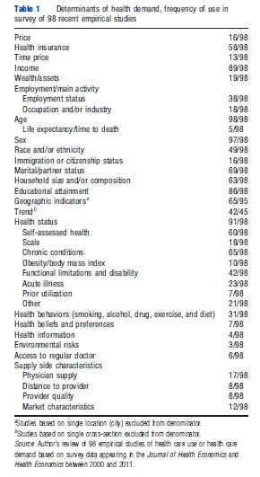
Appealing to the economic notion that the price of consuming health care extends beyond direct out-of-pocket costs to time, 13 of the 98 studies included time price. A typical direct measure of time price multiplies a person’s wage rate by the time they spend traveling to health care and wait time. In other cases, proxy measures such as travel time were used. Measures of income were almost always included (89 studies). In most cases, this was total family income divided by the square of the number of household members. This normalization assumes that the larger the family, the smaller the share of resources available to any one member. In a handful cases, wealth or household assets were used as a proxy for income. In 16 studies, wealth or assets were included in addition to income. The theory here is that consumers consider more than just current income.

Although widely available in surveys, employment status (38) and/or information about occupation or industry (18) were included in a minority of studies. These are choice variables that do not directly determine health as per the theoretical models of health demand. A major concern here is reverse causality. Poor health might lead to job loss, and thus employment-related variables will reflect some aspects of health. Reasons for including employment characteristics might be that certain industries and occupations carry greater health risks from accidents, exposure to hazardous materials, or stress. They might also proxy for preferences about health care. In the United States, industry, occupation, and firm size are also correlated with generosity of insurance and access to paid sick leave.

Health And Health-Related Determinants

Direct measures of individual health were included in 91 of the 98 studies. They were uniformly powerful predictors of use. Reflecting the multidimensional nature of health, a wide range of measures was used. The most common were chronic health conditions such as diabetes, asthma, and heart disease (65 studies). Some studies used counts of chronic conditions, others each individual condition. The next most common health status measure were variants of a single-item self-assessed health status scale (60) asking respondents to rate their health (e.g., excellent, good, fair, and poor). A number of studies (42) included measures of disability or functional limitations such as difficulty walking upstairs or lifting. These were more common in studies of older populations. Other studies included measures derived from longer health-rating scales (18), acute illness or symptoms such as fever (23), measures related to obesity (10), and a variety of other measures (21).

All measures of health status raise concerns about reverse causality. Choices of which measures to include are driven by a combination of availability and an individual researcher’s beliefs about the trade-offs between relevance in determining demand and potential bias. Chronic conditions are appealing because their very nature makes them less prone to concerns that current health care use changes whether an individual has the condition or not. For example, once you have diabetes you always have diabetes; treatment manages symptoms. Bias is a greater concern with acute symptoms of illness explaining why they are less commonly used, even though it is believed that they drive much use. Acute illness was more commonly included in studies based in low-income countries, where the balance between bias and relevance may be different.

Prior health utilization is a strong predictor of current health care use, and seven studies appeared to include it for this reason. If we are simply interested in obtaining the best possible predictions of current health care use, this is fine. However, if we are interested in the extent to which health explains health care use, it is not fine. For example, if a person has consumed lots of health care in the previous year because of his/her diabetes, then the intensity would also continue the year ahead. Henceforth, the effect estimated for diabetes is diminished. By including last year’s use, the estimate for diabetes is greatly diminished.

Seven studies included no measures of health status. In two of them, none were available. The remainder explicitly or implicitly excluded health because of potential endogeneity. The researchers are making the call that the bias introduced by including health is worse than the omitted variables bias created by excluding a powerful determinant. Most make the call the other way.

Another set of health-related determinants commonly included are smoking, alcohol and drug use, exercise, diet, and other health behaviors (31 studies). Many researchers exclude them because they are choices related to health. However, they are also often strongly related to use. For example, a history of smoking can lead to significant health problems today even if one does not currently smoke.

Access And Supply-Side Determinants

Six studies included whether a person has access to a regular medical provider. Although often available, most researchers omit this as a choice variable because of its clear endogeneity with health care use. A larger number of studies included local area physician, hospital or other provider supply (17), distance to provider (8), or market characteristics (12) such as managed care concentration. These are generally used as proxies for availability and access to providers. Some may also proxy for time price. Many researchers omit these because observed health care use is a simultaneous function of supply and demand (though rarely modeled this way) making supply-related variables endogenous.

Demographic Determinants

Among the demographic variables, age and sex appear universally. Five studies used life expectancy (or time to death) in addition to or in place of age, arguing that life expectancy is a stronger predictor of health care use. A number of studies included interaction terms between age and sex, allowing for the effects of age to vary with sex, and vice versa. A few ran separate models stratified by sex, allowing for the effects of all determinants to vary by sex. Measures of race, ethnicity, or cultural group were included in 49 of the studies. Studies without such measures tended to come from countries with more homogenous populations. Education status (number of years or degrees) was almost universal. Similarly, most included some combination of marital status and/or household composition (e.g., number of family members). More than two-thirds of the studies included geographic indicators such as locality and/or living in an urban or rural area.

Finally, almost all the studies that used data pooled across more than 1 year included some time or trend dimension in the model. With health care use generally increasing over time, it is important to capture overall shifts in health care demand.

Other Considerations

Table 1 describes the range of determinants included in empirical demand studies. In aggregate, some are used more regularly than others. The table does not capture that the studies reviewed varied considerably in how parsimonious or expansive the set of demand determinants included in each study were. This ranged from as few as six variables to as many as 87. In some cases, parsimony may be driven by computational demands. Some econometric methods are also fragile when including too many closely related variables. Often, though, individual researchers simply prefer more parsimonious models. If we are interested in only one or two determinants and a model with just a few variables captures these well, we may be okay omitting other potential determinants. However, if the omitted characteristics are correlated with these key determinants, our estimates will be biased.

Empirical Determinants Of Health Care Demand: An Illustration

The important roles that various theoretically derived and proxy determinants play in empirical models are illustrated using an example drawn from the author’s own work on the demand for mental health treatment. Specifically, treatment related to depression are examined. Depressive disorders are a group of chronic, but episodic diseases affecting millions of Americans. The effects that health, economic, and sociodemographic determinants have on the use of three treatment options for the treatment of depression are examined: nonspecialty visits (generally to primary care providers), specialty visits (psychiatrists, psychologists, and social workers), and antidepressant medications. Aside from obvious convenience, this example has been chosen to illustrate how empirical determinants can vary across different types of treatment. This depression treatment example also conveniently illustrates the difference between need for treatment and individual demand.

Being consistent with the literature, it is not attempted to jointly estimate demand and supply. The dependent variable in the models is observed utilization and is assumed to be equivalent to demand. The empirical example in other respects is simplified. First, using probit equations; it is only modeled whether a person used each type of treatment and not quantities. Second, it is not attempted to jointly model other aspects of consumer decision making (e.g., other goods and services, income, and employment). Third, the main estimates presented do not correct for potential endogeneity of health insurance, income, and health status.

The rules of thumb described above can help guide both selection of empirical determinants and their interpretation using this example.

Data

The data are drawn from the Medical Expenditure Panel Survey (MEPS), a large nationally representative household survey conducted annually in the United States since 1996 by the Agency for Healthcare Research and Quality. The MEPS contains a rich array of information on each household member’s health care use and expenditures, health insurance coverage, employment and income, health status and health conditions, and other sociodemographic characteristics. The MEPS is widely used to model the demand for health and to plan and evaluate health policy reforms and changes.

The MEPS utilizes an overlapping panel design to represent the civilian noninstitutionalized population in each calendar year. Households are interviewed in-person for five rounds covering 2 full calendar years. The average recall period for these five rounds is approximately 5 months. Generally, one person responds for all members of the household. In-person interviews are supplemented with self-administered health questionnaires (SAQs) of every adult to assess health status and experiences of care that might not be reliably captured by proxy. Follow-back surveys of physicians, hospitals, home health agencies, and pharmacies are used to collect more detailed information on health care spending and prescription medications.

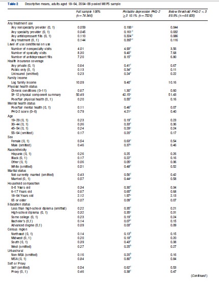
Current sample sizes for each panel are approximately 7500 households and 18 000 individuals. The analytic sample used here is drawn from the 2004–08 panels of the MEPS and includes 37 173 adults aged 18–64 with two observations each with complete information on treatment use, depression status, and other covariates.

Analyses

Table 2 presents means of the dependent variables and all demand determinants for the full sample and also stratified by an indicator for probable depression. Departing from standard practice, the specification of each demand determinant and its rationale for inclusion one by one with the results and interpretation from the empirical demand model are described.

 

Economic Determinants: Specification, Results, And Interpretation

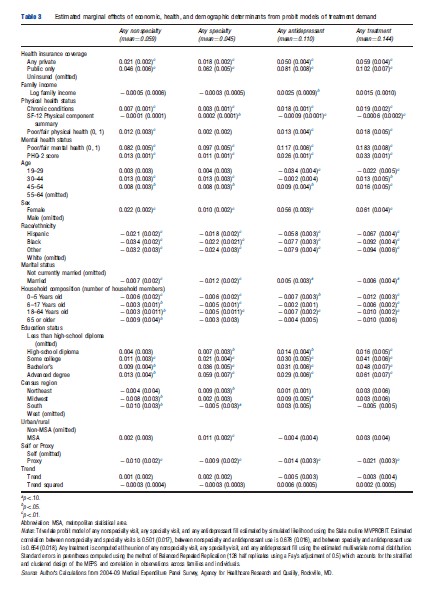
Table 3 presents the empirical estimates of the effects of economic, health status, and sociodemographic determinants from three probit equations describing any nonspecialty, specialty, and antidepressant use. The table adds a fourth column, which computes the combined effect of each determinant on the use of any of the three types of treatment. To ease in the interpretation of magnitudes, marginal effects are presented instead of coefficient estimates. For binary indicators, the marginal effects represent the change in the expected probability of using treatment for that group compared to the omitted group. For example, the marginal effect of 0.022 females for nonspecialty services implies that women are 2.2% points more likely to have nonspecialty mental health visits than men. The overall mean use of nonspecialty treatment is 5.9%, men and women combined, so this represents a substantial differential. For continuous measures, the marginal effect represents the change in the probability of use for a one unit change. For example, each additional child in a household less than 6 years (marginal effect = 0.006) is associated with a 0.6% point decrease in the use of nonspecialty care.

Health Insurance

Like many surveys, price is only observed in the MEPS among users. Deriving theoretically consistent prices suitable for demand estimation from these partial observations is conceivable but difficult. Health insurance is used as a proxy instead. The MEPS contains extensive insurance coverage information. For simplicity, a three category summary of insurance status provided on the MEPS public use file (INSCOV) is used. In the sample of adults aged 18–64 years, 23% were uninsured the entire calendar year, 64% had private insurance (mainly through employers or unions) for all or part of the year, and 13% had public insurance only, mainly Medicaid or Medicare (Table 2).

It is seen that private and especially public insurance are strongly correlated with treatment. For example, people with public insurance are 10.2% points more likely to use any type of treatment than people without insurance. Although we expect positive effects of insurance on use, there are reasons to believe the estimated magnitudes are too large. First and foremost is adverse selection. Second, public health insurance may proxy in part for unmeasured severity of depression because both Medicare and Medicaid, in part, serve as disability programs. The qualifying process itself, which includes clinician diagnoses, may differentiate between levels of depression in ways that move beyond a limited depression scale. Using first month insurance indicators instead of full-year insurance to minimize postdiction bias does little to magnitudes. However, when the model is reestimated explicitly accounting for the potential endogeneity of insurance, the estimated effects of public and private insurance drop by half (not shown).

Income

Income is included as a theoretically important determinant but discussion on its interpretation has been brief. Following common practice, the log of total family income is divided by the square root of the number of household members. Positive income effects are generally expected, but for antidepressant use, only a small effect is observed. Income may be confounded with unobserved depression severity and other factors. For example, depression often leads to job loss, thereby biasing downward the effects of income.

Health And Mental Health Determinants: Specification, Results, And Interpretation

Physical Health

Three widely used measures of physical health are included from an earlier review. A strong correlation between depression and physical health has long been observed but the causal pathways remain unclear. Certain medical conditions, for example, heart attack, may lead to or exacerbate depression. Or patients might simply be depressed about physical ailments, especially if they lead to job loss or other life changes. On the other side of the equation, depression may lead to poor diet and exercise. In the course of treating people for physical ailments, providers might also detect depression leading to more care.

The first measure is a simple count of a set of 11 chronic conditions that are ascertained in each MEPS panel. Respondents are asked if the doctor ever told the person they had diabetes, arthritis, asthma, emphysema, stroke, high blood pressure, high cholesterol, coronary heart disease, heart attack (myocardial infarction), angina, and any other heart disease. A graph of the 0–11 condition count versus treatment was approximately linear (not shown). The regression results in Table 3 show a strong association between chronic conditions and antidepressant use in particular, with each additional condition increasing the probability of antidepressant use by 1.8% points. The association is used here because, even with reverse causality minimized, these chronic conditions are still likely correlated with depression severity, not captured in the depression index.

The second measure is the physical health summary score from the Short Form-12 (SF-12) contained in the MEPS Adult SAQ asked in the middle to later part of each calendar year. The SF-12 is a well-validated health inventory containing 12 questions on a number of dimensions of physical and mental health symptoms and functioning. This composite index is scaled from 0 to 100 and normalized to approximately 50 with a higher score indicating better health. The effect on nonspecialty use was not significant. Better physical health is associated with a reduced probability of antidepressant use as expected. Curiously, better physical health, controlling for chronic conditions and perceived health status, is associated with a small but statistically significant increase in specialty use.

The third physical health measure is derived from the standard 1-item perceived health status question asked in each of the five rounds of MEPS. Respondents are asked relative to persons their age, whether each member of the household is in excellent, very good, good, fair, or poor health. The poor and fair responses in either of the first two rounds during a calendar year into a single binary indicator (ever poor or fair vs. good/very good/excellent) have been combined. Turning to the actual results in Table 3, there is an independent effect of poor or fair perceived health on treatment, increasing the likelihood of nonspecialty visits by 1.2% points and antidepressant use by 1.3% points.

The SF-12 and poor/fair health measures bring the potential for obvious reverse causality problems because they are measured contemporaneously with treatment. In fact, they could be measured well after treatment if treatment occurred earlier in the year. Using the strategy of minimizing postdiction by measuring health at the earliest possible point during the year or using prior year values, alternative ways of constructing and using these variables have been tested. For the poor/fair measure, the round 1 responses are used only to construct an alternate poor/fair indicator. This had no appreciable effect on magnitudes of the effects. Because the SF-12 is measured later in the year, the first year of each person’s observations has been discarded but used their SF-12 (and poor/ fair health status) from the first year to estimate the demand models on the second year’s observations. Again, nothing changed. Rather than lose half the observations, it has been opted to keep the models as they are.

Interpretation of all three physical health status measures is uncertain because they are likely associated with unmeasured aspects of health and preferences . To test this, a version of the demand models presented here has been estimated, which explicitly accounts for these potential correlations. The results (not shown) suggest that the physical health measures indeed are correlated with unmeasured aspects of people’s health and preferences toward care, substantially reducing the magnitudes of the observed effects of the three measures.

The MEPS contains a number of other measures related to functional limitations and disability, recent symptoms associated with chronic and other diseases, measures of work or school days lost and bed days, and a number of other adult health measures as well as measures specific to children and adolescents. Good arguments could be made for including any one of a number of them. The main reason for sticking with just chronic conditions, SF-12, and perceived health status is parsimony. Together they do a reasonable job of representing physical health and capture many of the same dimensions of the other measures in this context.

Mental Health Status

Conceptually, we might think mental health is the most important determinant of demand. If you are depression free, why seek treatment? Thus, the 2-item Patient Health Questionnaire (PHQ-2), a well-validated depression screener taken from the Adult SAQ, is included. The PHQ-2 asks ‘‘Over the last 2 weeks, how often have you been bothered by any of the following problems?’’ ‘‘Feeling down, depressed, or hopeless,’’ and ‘‘little interest or pleasure in doing things.’’ Responses ranged from ‘‘not at all’’ (0) to ‘‘nearly every day’’ (3). A score of 3 or higher is suggested as a cut-point for depression screening. The linear PHQ-2 scale (0–6) is used because it measures both probable clinical depression (PHQ- 2≥3) and severity. For example, each increment in the 0–6 scale is associated with a 2.6% point increase in antidepressant use.

The mental health analog of perceived physical health status is also included. Even controlling for symptoms of depression, we find that perceived poor or fair mental health increases nonspecialty use by 8.2% points, specialty use by 9.7% points, antidepressant use by 11.7% points, and any treatment by 18.3% points compared to those with better mental health.

Two concerns with the PHQ-2 and perceived mental health measures are noted. Most importantly, the first information we get about depressive symptoms occurs later in the first year a person enters the MEPS, and the PHQ-2 scale asks only about symptoms in the past 2 weeks. If a person sought treatment in the past because of depression, assuming treatment works, he/she may be symptom free by then. This will tend to reduce the impact of depression estimated. Like physical health, an alternative has been tested using only the second year of data for each person substituting their first year PHQ-2 measurement and perceived mental health status. Surprisingly, no appreciable differences in the effects on treatment use have been found. This may be because, although depression is a chronic illness, it is also episodic. It is also possible that reverse causality bias is offset by people with depression in the first year who do not carry symptoms into the second year and do not need treatment. However, as with physical health status, when the demand models were reestimated to explicitly account for endogeneity bias, the effects of mental health status were substantially reduced.

Second, although the PHQ-2 does a nice job for a two-item scale, it is not as sensitive to depression severity as its longer cousin the PHQ-9 or other depression instruments. A more sensitive depression measure would reduce the potential for our health insurance and demographic determinants to be confounded with unobserved severity of mental health.

Sociodemographic Determinants: Specification, Results, And Interpretation

Age

Age is represented by four binary indicators: ages 19–29, 30–44, 45–54, and the omitted category 55–64 years. For specialty and nonspecialty care, there is an upside down Ushaped relationship between age and use with the peak in the age 30–44 years range. In both, those aged 30–44 years are 1.3% points more likely to use treatment compared to those aged 55–64 years and approximately 1.0% points more likely than those aged 19–29 years. Antidepressant use showed a different pattern with respect to age with use peaking in the 45–54 year old group.

What do these U-shaped relationships mean? Age, in part, serves as a proxy for health and mental health not captured in our health measures. But other explanations are plausible. Young adults cumulatively have less exposure to the health care system, and thus, less time for providers to detect depression and recommend treatment. Tastes and preferences may change as young adults mature, or alternatively, they may suffer for years before seeking treatment. Cohort effects may also be at play here with stigma likely greater in older groups.

Sex

Sex is usually included in demand models to reflect biological differences in the prevalence, course, and severity of disease. Women, for example, are much more likely to have depression. However, controlling for symptoms of depression as much as possible in the MEPS, we find that women are still much more likely than men to use treatment, especially antidepressants. Whether this is due to unmeasured differences in depression between men and women or differences in preferences over treatment or stigma we cannot say.

Race And Ethnicity

A standard representation of race and ethnicity was used in dividing the population into the following groups: non-Hispanic Whites (the omitted group), Hispanic ethnicity, Black race, and others including those of Asian and mixed race ancestry. Hispanics, Blacks, and others are substantially less likely to have nonspecialty and specialty mental health visits but proportionately even less likely to use antidepressants than Whites. For example, Blacks are almost 8% points less likely than Whites to use antidepressants controlling for other determinants. It is hard to see how unmeasured differences in depression severity might explain these magnitudes. More likely, it reflects unmeasured differences in attitudes and differential access to care. Here measures related to immigration and citizenship status have not been included because they are not available on the MEPS public use files, but they substantially reduce the magnitude of the effects for Hispanics on treatment use (not shown).

Marital Status And Household Composition

Following standard practice (Table 1), a measure of whether the person was married at the time of their round 1 MEPS interview is included. Counts of the number of household members between the ages of 0–5, 6–17, 18–64, and 65 years and older are also included. One reason for including household composition variables is the potential protective health benefits of marriage. Another is that increasing family size may reduce resources available, both money and time, to any one particular adult in the family for treatment. Consistent with both rationales, the measures were negatively correlated with different types of treatment use, with the exception of a small positive effect of marriage on antidepressant use. But interpretation here is difficult. Depression may also lead to divorce and family dissolution (reverse causality) reducing the magnitudes of the effects which have been observed. Family composition may also be related to unmeasured preferences for depression treatment.

Education

A series of binary indicators corresponding to degrees obtained is obtained: less than high-school diploma (omitted), high-school diploma or equivalent, some college, bachelors, and advanced degree (Masters, MD, JD, PhD). This simultaneously allows for a nonlinear relationship between education and treatment as well as potential ‘degree’ effects. That is, more than just another year or 2 years of college separates someone with some college from someone who earned their bachelor’s degree. Certainly, this is true in the labor market but may extend to preferences over treatment through its effects on social class and norms.

The regression results show substantial differences by education, even controlling for symptoms of depression. Those with a high-school diploma or less are substantially less likely to seek treatment than their better educated counterparts. Interestingly, there is little difference in use of nonspecialists and antidepressants among those with some college, bachelor’s, or graduate degree. However, there is a strong gradient for specialists, with use increasing sharply with education.

Clearly education is strongly related to depression treatment, but is it a determinant in a causal sense? Educated consumers might understand better the importance of adherence with antidepressant medication schedules. Or they may have higher quality interactions with therapists providing cognitive behavioral therapy (CBT). In both cases, better educated consumers might derive greater benefits and thus more likely to continue treatment. They may also be more likely to initiate treatment if they better understand potential benefits. However, we cannot help but suspect that unmeasured preferences and social class norms drive much of the educational differences we observe. It is hard to understand why those with graduate degrees would be so much more efficient than those with bachelor’s degree in the production of CBT and other talk therapies but not with antidepressant medication. More likely, the stigma surrounding seeing psychiatrists, psychologists, and other specialists is lower among those with graduate degrees.

Reverse causality is potentially a problem with our education measures. Depression may begin in adolescence leading to lower educational achievement through decreased motivation. Such bias would tend to reduce the magnitude of educational effects measured. In the opposite direction, higher education may be correlated with greater economic resources available to pay for treatment.

Geography

Indicators for each of the four Census Regions in the United States (Northeast, Midwest, South, and West) and whether the person resided in a Census Bureau defined Metropolitan Statistical Area, a measure of whether the person lives in an urban or rural area have been included. These are likely correlated with tastes for treatment. For example, stigma for mental health treatment is thought to be stronger in rural areas and in the South. They are also attractive proxies because bias from reverse causality (health causes location) is probably small. Indeed, we find that those in urban areas are more likely to use specialists, whereas those in the South are somewhat less likely. Geography may also be correlated with availability of health care services, but it is also likely that supply follows demand (more doctors in areas where people like to use services). A growing literature also suggests substantial local variations in medical provider practices. In this context, there may be variations in preferences among psychiatrists to treat patients with talk therapy instead of medicating depressed patients.

Proxy

The MEPS is a household survey with one person responding for all household members (the Adult SAQ is one exception). Although MEPS requests that this be the person most knowledgeable about health and health care in the family, there may still be issues with proxy responses. For example, a wife may not be aware that her husband sought depression treatment. To account for the potential for underestimating treatment use obtained by proxy, an indicator is included for whether the MEPS sample member is the respondent (proxy = 0) or not (proxy = 1). Consistent with this worry, the regression results show that proxy respondents are approximately 1% point less likely to use each of the three types of treatment. Of course, proxy status could be correlated with other unmeasured aspects of individuals related to treatment.

Trend

To account for the possibility that demand increased between 2004 and 2009, two time-trend variables were included. The first is linear term for survey year (minus 2004 to normalize to 0). The second term squares the first allowing for nonconstant changes in demand. In fact, there is no discernable trend in overall demand using this or any number of alternative specifications between 2004 and 2009. This would not have been true in the late 1980s and 1990s when demand grew rapidly with the introduction of new classes of antidepressants.

Excluded Determinants

A number of potential determinants do not appear in this empirical example. Employment status, occupation, and industry have been excluded because of their direct potential for reverse causality and uncertain effects on demand. Ideally, time price would be included, but direct measures of travel and time costs as well as suitable proxies are lacked. The MEPS Adult SAQ contains four items designed to represent individual attitudes and beliefs. However, the correlation between first and second year responses was lower than expected suggesting responses may be endogenous with current health and health care use. Good arguments could be made either way for including smoking status, but it has been excluded as lacking a clear a priori hypothesis about its effects. Although clearly relevant to depression, alcohol and drug behaviors are not available. A number of available access measures believed to be endogenous have been omitted. Finally, Local area supply side and market characteristics that can be merged onto MEPS for similar reasons have been omitted.

Need Versus Demand: Illustrating With The Empirical Example

Policymakers and advocates often speak of ‘unmet need’ for treatment for diseases such as diabetes, heart disease, and depression. In this context, need is some norm that is being applied to groups of individuals defined by illness and then determining the extent to which they actually receive care. In the example given, if a diagnosis of depression is used as the determinant of need then it is being said that all individuals with depression should receive treatment. Those without it have unmet need. If one prefers, the definition can be made more restrictive, as many have proposed, to include additional functional impairment criteria, but regardless we are still applying some external norm. Alternatively, the actual use of individuals in one group (say high income) as a norm for other groups can be used.

As introduced earlier, economists view demand strictly through the eyes of the individual. Even in demand–supply graphs, market demand curves are simply the sum of individual demands. The authors talk about ‘need’ variables being included in demand models, but individuals take this more into account than just their health in determining whether and how much care to consume. An individual with depression may or may not perceive that they need treatment at all. Some depressed individuals may not seek treatment even if their out-of-pocket price is zero. For others, whether they seek treatment may depend critically on price.

Survey data such as MEPS gives us the opportunity to study measures of ‘need’ as distinct from demand and use. If we look at the descriptive statistics on Table 2, we see that only 40% of people with a current PHQ-2 score of 3 or greater (suggesting probable depression and the need for further screening) receive treatment. If we use this cut-point as our norm for treatment need, it suggests that more than half of currently depressed individuals do not receive treatment and therefore have unmet need. Conversely, 12% of those not meeting our hypothetical norm for need consume treatment. The empirical model can be used to simulate the effect that changing a key determinant has on changing the relationship between our norm for need and actual demand. Health insurance coverage, because it is so amenable to policy changes, is the obvious choice. Here, the model implies that providing public coverage to all of the uninsured would reduce the gap between need and demand in the uninsured from 78% to 65% and among all adults aged 18–64 years from 60% to 57%.

Conclusion

Specifying and interpreting the empirical determinants of health care demand is as much art as science. As seen from the author’s review of recent empirical studies, there is not only widespread agreement about some determinants such as age, sex, health status, and education but also wide variation in the treatment of other characteristics that might be correlated with health care use. Researchers are confronted with tough trade-offs among competing concerns in selecting and specifying determinants they think relevant in demand models. Formal models of health care demand can help guide us about the treatment of variables such as health status, income, and price. Theory also guides us in the choice of proxies and, also using statistical principles, how to best specify these proxies to represent unmeasured aspects of health and treatment seeking preferences . As seen from the empirical illustration, proxies such as education are often powerful predictors of demand. These same economic and statistical principles also aid us in interpreting our empirical determinants. But in a world where unobserved preferences and health play such a key role, we will always face some uncertainty about how to model the empirical determinants of health care demand.

Disclaimer

The views expressed in this article are those of the author, and no official endorsement by the Agency for Healthcare Research and Quality, or the Department of Health and Human Services is intended or should be inferred.

Bibliography:

1. Coffey, R. M. (1983). The effect of time price on the demand for medical-care services. Journal of Human Resources 18, 407–424.
2. Cook, B. L., McGuire, T. G. and Zaslavsky, A. M. (2012). Measuring racial/ethnic disparities in health care: Methods and practical issues. Health Services Research 47, 1232–1254.
3. Deb, P. (2001). A discrete random effects probit model with application to the demand for preventive care. Health Economics 10, 371–383.
4. Freiman, M. P. and Zuvekas, S. H. (2000). Determinants of ambulatory treatment mode for mental illness. Health Economics 9, 423–434.
5. Garfield, R.L, Zuvekas, S. H., Lave, J. R. and Donohue, J. M. (2011). The impact of national health reform on adults with severe mental disorders. American Journal of Psychiatry 168, 486–494.
6. Kenkel, D. S. (1990). Consumer health information and the demand for medical care. Review of Economics and Statistics 72, 587–595.
7. Manning, W. G., Newhouse, J. P. and Ware, J. E. (1982). The status of health in demand estimation; or, beyond excellent, good, fair, poor. In Fuchs, V. R. (ed.) Economic aspects of health, pp. 143–184. Chicago: University of Chicago Press. Available at: http://www.nber.org/books/fuch82-1 (accessed 24.06.12).
8. Meyerhoefer, C. D. and Zuvekas, S. H. (2010). New estimates of the demand for physical and mental health treatment. Health Economics 19, 297–315.
9. Propper, C. (2000). The demand for private health care in the UK. Journal of Health Economics 19, 855–876.
10. Rous, J. J. and Hotchkiss, D. R. (2003). Estimation of the determinants of household health care expenditures in Nepal with controls for endogenous illness and provider choice. Health Economics 12, 431–451.
11. Sosa-Rub´ıa, S. G., Gala´rraga, O. and Harris, J. E. (2009). Heterogeneous impact of the ‘‘Seguro Popular’’ program on the utilization of obstetrical services in Mexico, 2001–2006: A multinomial probit model with a discrete endogenous variable. Journal of Health Economics 28, 20–34.
12. Wagstaff, A. (1986). The demand for health: Some new empirical evidence. Journal of Health Economics 5, 195–233.
13. Yang, Z., Gilleskie, D. B. and Norton, E. C. (2009). Health insurance, medical care, and health outcomes. Journal of Human Resources 44, 47–114.
14. nimh.nih.gov National Institute of Mental Health, National Institutes of Health.
15. meps.ahrq.gov Medical Expenditure Panel Survey (MEPS) On-Line Resources and Data, Agency for Healthcare Research and Quality.